It may be time to reconsider weather variables as instruments

For many years, I was sceptical of instrument variables analysis. I expressed a little of this scepticism in one of my early posts on this blog in 2014. However, by then I was starting to come around to the idea, and encouraging my PhD students to consider using it in their work. However, I may have been shifted a little more back towards scepticism by this new working paper by Jonathan Mellon (West Point).

Mellon focuses on the use of weather variables as instruments, and demonstrates the problems associated with using them. However, before he gets that far, he has a very clear exposition of what instrumental variables entails, which is worth sharing. First, here's Figure 1 from the paper:

Then, the associated explanation:

Endogeneity is one of the most pervasive challenges faced by social scientists. Naively, we might assume the causal relationship between two social science variables 𝑋 and 𝑌 can be estimated by their observed relationship [first panel of Figure 1]... However, social scientists usually doubt this simple picture and believe most variables share unmeasured confounders 𝑈 (second panel). One strategy for conducting causal analysis in the presence of endogeneity is using an instrumental variable 𝑊 that causally affects 𝑋 but is uncorrelated with the error term... One of the most important assumptions for any instrumental variable estimation is the exclusion restriction that 𝑊 is associated with 𝑌 only through its relationship with 𝑋 (i.e. there are no other causal pathways from 𝑊 to 𝑌). The assumed DAG for the IV estimation is shown in figure 1’s third panel...

The fourth panel of Figure 1 also demonstrates a problem, where the instrumental variable W affects some other variable Z, which in turn has a direct effect the outcome variable Y.

Mellon's contribution in this paper is to draw attention to the fact that weather variables (mainly rainfall, but also other variables like temperature, wind speed or direction, sunlight, or various others) have been used in so many applications as the variable W, that they must surely have effects on almost every outcome variable Y that don't run only through the variable X. It's kind of an obvious point when you think about it, and Mellon uses the results from over 150 papers to illustrate it, concluding that:

Cunningham (2018) argues that a good instrument should have a “certain ridiculousness”. Until the secret endogenous route to causation is explained, the link between the instrument and outcome seem absurd. In a world where Australians and Californians cannot leave their houses for months at a time due to forest fires, and 1-3 billion people are projected to be left outside of historically-habitable temperature ranges... linkages between weather and the social world are just not ridiculous enough.

Mellon uses weather instruments as his example, but the point he is making is broader. We need to be much more critical of the instrumental variables that are employed. He even offers a simple literature-search-based algorithm for determining whether a proposed instrumental variable is likely to fail the exclusion restriction, which can be used alongside the usual theoretical justification for its use. 

Certainly, it is time to reconsider whether weather variables are valid instruments. Only time (and further criticism along the lines that Mellon has advanced) will determine whether we should be equally sceptical of instrumental variables analysis more generally.

[HT: Marginal Revolution]

The impact of remote learning in Brazilian high schools

Last week, I wrote a post expressing some frustration with a paper that purported to show the effect of online teaching on student learning, but really only showed the effect of online revision materials. I lamented that:

We do need more research on the impacts of online teaching and learning. However, this research needs to actually be studies of online teaching and learning, not studies of online revision.

Now, this new article by Guilherme Lichand, Carlos Alberto Doria, Onicio Leal-Neto (all University of Zurich), and João Paulo Cossi Fernandes (Inter-American Development Bank), published in the journal Nature Human Behaviour (open access) is much more of what I was looking for, and what we need. Lichand et al. look at the effect of the lockdown-induced shift to remote learning on students in high schools in São Paulo State, Brazil. They follow a similar difference-in-differences strategy to the paper I referred to last week, but instead of comparing students from schools with different access to materials, before and during the pandemic lockdowns, they compare students' performance between the first quarter and fourth quarter of the school year in 2020 (when the lockdowns were in place for the last three quarters) with 2019 (when there were no lockdowns). Their data covers over 8.5 million quarterly observations of 2.2 million students enrolled in sixth through twelfth grades. That also allows Lichand et al. to do a further comparison between students in middle schools and high schools, because:

...some municipalities allowed in-person optional activities (psycho-social support and remedial activities for students lagging behind) to return for middle-school students and in-person classes to return for high-school students...

So, comparing middle school and high school students' performance in Q1 and Q4 between districts that did and did not allow a return to in-person classes for high school students (in a 'triple differences' model) allows a further test of the effect of in-person classes. However, the results on this latter analysis are not as robust, as Lichand et al. don't know precisely which schools went back to in-person schooling (only which districts would allow it). In both sets of analyses, their outcome variables are the risk of dropout, and standardised test scores (and they observe test scores for about 83.3 percent of the sample).

In the first set of comparisons, they find that:

...remote learning might have had devastating effects on student dropouts, as measured by the dropout risk, which increased significantly during remote learning, by roughly 0.0621 (s.e. 0.0002), a 365% increase (significant at the 1% level...)... this result is suggestive of student dropouts within secondary education in the State having increased from 10% to 35% during remote learning...

The differences-in-differences strategy, in turn, uncovers dramatic [learning] losses of 0.32 s.d. (s.e. 0.0001), significant at the 1% level, a setback of 72.5% relative to the in-person learning equivalent.

Those are some huge negative effects of remote learning. Turning to the second comparison, of the effect of returning to in-person classes on student learning, they find:

...positive treatment effects on learning, fully driven by high-school students. In municipalities that authorized high-school classes to return from November 2020 onwards, test scores increased on average by 0.023 s.d. (s.e. 0.001, significant at the 1% level...), a 20% increase relative to municipalities that did not.

So, students managed to recover over half of the learning losses when in-person classes resumed. This is the good news part of this paper, especially since:

In municipalities that authorized schools to reopen for in-person academic activities in 2020, the average school could have done so for at most 5 weeks.

So, it didn't take long to erase much of the negative impact of remote teaching on learning. However, there was no significant effect on dropout risk, so presumably students who were likely to drop out did not reconsider their choice once schools had returned to in-person instruction.

The evidence is becoming clearer, and these results are in line with those from the literature on university-level students. Remote teaching has had a substantial negative effect on student learning. However, what was missing from this paper was an analysis of the heterogeneous effects between good students and not-so-good students. I expect that the dropout risk, and probably the learning losses, were heavily concentrated in the latter. What would have been most interesting would be whether the recovery in learning after the return to in-person teaching was also concentrated among the low-performing students. Perhaps future studies will help to reveal that.

Read more:

• Online vs. blended vs. traditional classes
• Flipped classrooms work well for top students in economics
• Flipped classrooms are still best only for the top students
• Online classes lower student grades and completion
• Online classes may also make better students worse off
• Meta-analytic results support some positive effects of using videos on student learning
• New review evidence on recorded lectures in mathematics and student achievement
• Meta-analytic results may provide some support for flipping the classroom
• The value of an in-person university education
• The pandemic may have revealed all we need to know about online learning
• Live streamed video lectures and student achievement
• Low-performing students, online teaching, and self-selection
• A slightly more optimistic take on online learning during the pandemic
• Research-based instructional strategies and flipped classrooms in economics
• Using microcommitments and social accountability to improve online and hybrid learning
• What pandemic schooling tells us about online learning
• We should be careful not to conflate the effect of online revision with the effect of online teaching

Gib delivery workers may be due for a payday

The New Zealand Herald reported last week:

Workers who deliver hundreds of tonnes of Gib to building sites across Auckland each day are striking for better pay.

About 40 truck drivers and labourers are picketing outside the Penrose base of the delivery company CV Compton.

They want an 11 per cent pay rise, but the company has offered much less...

It took time to train workers to deliver the plasterboard but they often lasted less than a week on the job because it was heavy labour, [Driver assistant James] Ramea said...

Gib was in demand and those delivering the plasterboard were working hard, [First Union organiser Emreck Brown] said.

"Prices of Gib has increased in the last couple of years and this year it has increased significantly. We need some support from the company just to help the members who're helping the company."

In a search model of the labour market, each match between a worker and an employer creates a surplus, which is then shared between the worker and the employer. The share of the surplus (and hence, the wage for the job) will depend on the relative bargaining power of the worker and the employer. If the worker has relatively more bargaining power, then they will receive a higher share of the surplus, in the form of a higher wage.

In this case, there is reason to believe that the workers' bargaining power has increased. That isn't because "those delivering the plasterboard were working hard", or even because it takes "time to train workers to deliver the plasterboard but they often lasted less than a week on the job because it was heavy labour". Those factors likely haven't changed recently.

What has changed is two things. First, the unemployment rate is low. Low unemployment increases the relative bargaining power of workers, because if a worker leaves their job (or refuses an employment offer), the employer then has to start the process of searching for a new worker all over again. The employer would face the search costs of the time, money, and effort spent searching for a worker and evaluating potential matches.

Second, because the "Prices of Gib has increased in the last couple of years", the value that the workers create for the employer have increased. That in itself doesn't affect wages in a search model of the labour market (although it does in a supply and demand model, where the demand for labour is based on the value of the marginal product of labour). However, because the workers are threatening to strike, the costs of the strike to the employer are likely higher because of the high value of gib deliveries foregone. That also increases the relative bargaining power of the workers.

None of this is to say that the gib delivery workers are going to see a huge increase in their wages. Employers tend to retain most of the bargaining power. However, the gib delivery workers have a bit more bargaining power than they would have had until relatively recently, and should be able to leverage that additional bargaining power for better wages and conditions.

The South Korean kimchi crisis

The Washington Post reported this week (possibly paywalled for you):

In the foothills of the rugged Taebaek range, Roh Sung-sang surveys the damage to his crop. More than half the cabbages in his 50-acre patch sit wilted and deformed, having succumbed to extreme heat and rainfall over the summer.

“This crop loss we see is not a one-year blip,” said Roh, 67, who has been growing cabbages in the highlands of Gangwon province for two decades. “I thought the cabbages would be somehow protected by high elevations and the surrounding mountains.”

With its typically cool climate, this alpine region of South Korea is the summertime production hub for Napa, or Chinese cabbage, a key ingredient in kimchi, the piquant Korean staple. But this year, nearly half a million cabbages that otherwise would have been spiced and fermented to make kimchi lie abandoned in Roh’s fields. Overall, Taebaek’s harvest is two-thirds of what it would be in a typical year, according to local authorities’ estimates.

The result is a kimchi crisis felt by connoisseurs across South Korea, whose appetite for the dish is legendary. The consumer price of Napa cabbage soared this month to $7.81 apiece, compared with an annual average of about $4.17, according to the state-run Korea Agro-Fisheries Trade Corp.

The effects of poor weather on the markets for cabbage and kimchi can be easily analysed using the supply and demand model that my ECONS101 class covered the week before last. This is shown in the diagram below. Think about the market for cabbage first. The market was initially in equilibrium, where demand D0 meets supply S0, with a price of P0 and a quantity of cabbage traded of Q0. Bad weather reduces the cabbage harvest, decreasing supply to S1. This increases the equilibrium price of cabbage to P1, and reduces the quantity of cabbage traded to Q1.

Now consider the market for kimchi. The costs of producing kimchi have increased. That leads to a decrease in the supply of kimchi. The diagram for the market for kimchi is the same as that for cabbage, with the equilibrium price increasing, and the quantity of kimchi traded decreasing. At least, that is the case for kimchi made from cabbage. Kimchi can also be made from other vegetables. The Washington Post article notes that:

The fermented pickle dish can also be made from radish, cucumber, green onion and other vegetables.

What happens in the markets for kimchi made from radishes? That is shown in the diagram below. Radish kimchi is a substitute for cabbage kimchi. Since radish kimchi is now relatively cheaper than cabbage kimchi, some consumers will switch to using radish kimchi. The effect is shown in the diagram below, where the radish kimchi market is initially in equilibrium with a price of PA, and a quantity of radish kimchi traded of QA. This increases the demand for radish kimchi from DA to DB, increasing the equilibrium price of radish kimchi from PA to PB, and increasing the quantity of radish kimchi traded from QA to QB.

The South Korean kimchi crisis is echoing through all types of kimchi, even if it is just the cabbages that are affected.

[HT: Marginal Revolution]

Is the Australian egg market demonstrating a cobweb pattern?

Last month in The Conversation, Flavio Macau (Edith Cowan University) wrote an interesting article about the egg market in Australia:

Australia is experiencing a national egg shortage. Prices are rising and supermarket stocks are patchy. Some cafes are reportedly serving breakfast with one egg instead of two. Supermarket giant Coles has reverted to COVID-19 conditions with a two-carton limit.

It's worth thinking about what has gotten Australia into this situation. Macau notes that:

Between 2012 and 2017, free-range eggs’ share of the market grew about 10 percentage points, to about 48%. Growth in the past five years has been half that.

But with more rapid growth predicted, and the promise of higher profits, many egg farmers invested heavily in increasing free-range production. In New South Wales, for example, total flock size peaked in 2017-18.

Like many agricultural industries where farmers respond to price signals and predictions, this led to overproduction, leading to lower prices and profits. This in turn led to a 10% drop in egg production the next year.

Now, consider the market for free range eggs, as shown in the diagram below. Demand increased substantially from 2012 to 2018, which is shown by the increase in demand from D0 to D1 (from Time 0 to Time 1). That pushed the price of eggs up from P0 to P1, and the quantity of eggs produced increased from Q0 to Q1 in response (the farmers increased production). Now, with the high price P1, farmers want to continue producing more eggs (Q2 for Time 2), but the demand has decreased back to where it was before (D2). [*] The quantity Q1 is now too many eggs, and to sell that many eggs, the farmers have to accept a lower price (P2). So, now they respond to the low price by cutting production to Q3 (for Time 3). But that level of egg production is too low, and the farmers are able to sell those eggs for the high price P3. Then, with the price high at P3, the farmers decide to increase production to Q4. And so on. Notice that this market is forming a cobweb pattern (following the red lines).

Now, is what we just described happening in the Australian egg market? Is there a cobweb model here? The cobweb model, as I have described before, relies on a key assumption: that the market has a significant production lag. Producers make their decisions about how much to produce today, but don't receive that production until some time in the future. This is a common feature of agricultural markets, but is it a feature of egg production? Chickens lay eggs every day (approximately), so when you consider it at that level, there is no production lag. Certainly, farmers don't have to wait long for eggs. However, the relevant production lag here isn't the production of eggs by chickens, it is how long it takes the farmers to respond to a change in price. If price falls, farmers may want to reduce the number of chickens they have, but that takes time (albeit, not a lot of time, since they can round up chickens and send them to a meat processor). If price rises though, farmers may want to increase the number of chickens they have, and that takes time, since they have to raise those chickens until they are ready to lay eggs. So, maybe there is half a production lag here - a lag in increasing production, but little lag when it comes to reducing production. So, this is not quite the cobweb model that I describe in my ECONS101 class (and as described for the diagram above). It does share some of the features of the cobweb, but only when prices are too low - it takes farmers more time to adjust to low prices than to adjust to high prices.

Australia finds itself in the uncomfortable position of having to wait for farmers to raise enough chickens so that egg production can increase. Once that happens, the market will adjust back to equilibrium (with a higher egg price).

*****

[*] Astute readers will note that the article only says that demand growth has fallen, rather than demand per se. However, if farmers are expecting high demand growth, and demand is less than farmers expected, that is similar to a decrease in demand. Not exactly, but close enough for our purposes.

We should be careful not to conflate the effect of online revision with the effect of online teaching

The pandemic forced education online, and should afford a lot of opportunity for us to understand the impact of online teaching on student engagement, student achievement, and student learning (and yes, those are all different things). Most of the literature on online learning relates to the university context, but students at university tend to be a little more self-directed than students at high school or below. What works in the university context doesn't necessarily translate to those other contexts, so we need more research on how online teaching affects high school and primary school students. I discussed one such paper back in May, which looked at students in Grades 3 through 8 in the US.

In a new article published in the journal China Economic Review (sorry I don't see an ungated version online), Andrew Clark (Paris School of Economics), Huifu Nong (Guangdong University of Finance), Hongjia Zhu (Jinan University), and Rong Zhu (Flinders University) look at the effects for three urban middle schools in Guangxi Province in China. These three schools (A, B, and C) each took a different approach to the government-enforced lockdown from February to April 2020:

School A did not provide any online educational support to its students. School B used an online learning platform provided by the local government, which offered a centralized portal for video content, communication between students and teachers, and systems for setting, receiving, and marking student assignments. The students’ online lessons were provided by School B’s own teachers. School C used the same online platform as School B over the same period, and distance learning was managed by the school in the same fashion as in School B. The only difference between Schools B and C is that, instead of using recorded online lessons from the school’s own teachers, School C obtained recorded lessons from the highest-quality teachers in Baise City (these lessons were organized by the Education Board of Baise City).

Clark et al. argue that comparing the final exam performance of students in Schools B and C with students in School A, controlling for their earlier exam performances, provides a test of the effect of online teaching and learning for these students. Then, comparing the difference in effects between School B and School C provides a test for whether the quality of online resources matters. There is a problem with this comparison, which I'll come back to later.

Clark et al. have data from:

...20,185 observations on exam results for the 1835 students who took all of the first 11 exams in the five compulsory subjects.

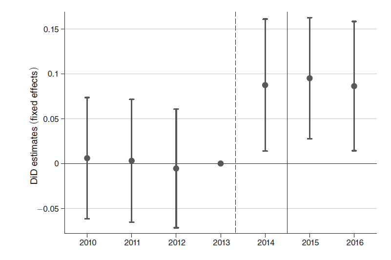
The five compulsory subjects are Chinese, Maths, English, Politics, and History. Clark et al. combine the results of all the exams together, and using a difference-in-differences approach (comparing the 'treatment group' of students from Schools B and C with the 'control group' of students from School A), they find that:

...online learning during the pandemic led to 0.22 of a standard deviation higher exam grades in the treatment group than in the control group...

And there were statistically significant differences between Schools B and C:

The online learning in School B during lockdown improved student performance by 0.20 of a standard deviation... as compared to students who did not receive any learning support in School A. But the quality of the lessons also made a difference: students in School C, who had access to online lessons from external best-quality teachers, recorded an additional 0.06 standard-deviation rise in exam results... over those whose lessons were recorded by their own teachers in School B.

Clark et al. then go on to show that the effects were similar for rural and urban students, that they were better for girls (but only for School C, and not for School B), and that they were better for students with computers (rather than smartphones) in both treatment schools. But most importantly, when looking across the performance distribution, they find that:

The estimated coefficients... at the lower end of distribution are much larger than those at the top. For example, the positive academic impact of School B’s online education at the 20th percentile is over three times as large as that at the 80th percentile. Low performers thus benefited the most from online learning programs. We also find that the top academic performers at the 90th percentile were not affected by online education: these students did well independently of the educational practices their schools employed during lockdown. Outside of these top academic performers, the online learning programs in Schools B and C improved student exam performance.

Clark et al. go to great lengths to demonstrate that their results are likely causal (rather than correlations), and that there aren't unobservable differences between the schools (or students) that might muddy their results. However, I think there is a more fundamental problem with this research. I don't believe that it shows the effect of online teaching at all, despite what the authors are arguing. That's because:

For students in the Ninth Grade, all Middle Schools in the county had finished teaching them all of the material for all subjects during the first five semesters of Middle School (from September 2017 to January 2020). Schools B and C then used online education during the COVID-19 lockdown (from mid-February to early April 2020 in the final (sixth) semester) for the revision of the material that had already been taught, to help Ninth Graders prepare for the city-level High- School entrance exam at the end of the last semester in Middle School.

The students had all finished the in-person instruction part of ninth grade by the time the lockdown started, and the remaining semester would have only been devoted to revision for the final exams. What Clark et al. are actually investigating is the effect of online revision resources, not the effect of online teaching. They are comparing students in Schools B and C, who had already had in-person lessons but were also given online revision resources, with students in School A, who had already had in-person lessons but were not given online revision resources. That is quite a different research question from the one they are proposing to address.

So, I'm not even sure that we can take anything at all away from this study about the effect of online teaching and learning. It's not clear what revision resources (if any) students in School A were provided. If those students received no further support from their school at all, then the results of Clark et al. might represent a difference between students who have revision resources and those who don't, or it might represent a difference between those who have online revision resources and those who have other revision resources (but not online resources). We simply don't know. All we do know is that this is not the effect of online teaching, because it is online revision, not online teaching.

That makes the results of the heterogeneity analysis, which showed that the effects are largest for students at the bottom of the performance distribution, and zero for students at the top of the performance distribution, perfectly sensible. Any time spent on revision (online or otherwise) is likely to have a bigger effect on students at the bottom of the distribution, because they have the greatest potential to improve in performance, and because there are likely to be some 'easy wins' for performance for those who didn't understand at the time of the original in-person lesson. Students at the top of the distribution might gain from revision, but the scope to do so is much less. [*]

We do need more research on the impacts of online teaching and learning. However, this research needs to actually be studies of online teaching and learning, not studies of online revision. This study has a contribution to make. I just don't think it is the contribution that the authors think it is.

Read more:

• Online vs. blended vs. traditional classes
• Flipped classrooms work well for top students in economics
• Flipped classrooms are still best only for the top students
• Online classes lower student grades and completion
• Online classes may also make better students worse off
• Meta-analytic results support some positive effects of using videos on student learning
• New review evidence on recorded lectures in mathematics and student achievement
• Meta-analytic results may provide some support for flipping the classroom
• The value of an in-person university education
• The pandemic may have revealed all we need to know about online learning
• Live streamed video lectures and student achievement
• Low-performing students, online teaching, and self-selection
• A slightly more optimistic take on online learning during the pandemic
• Research-based instructional strategies and flipped classrooms in economics
• Using microcommitments and social accountability to improve online and hybrid learning
• What pandemic schooling tells us about online learning

*****

[*] This is the irony of providing revision sessions for students - it is the top students, who have the least to gain, who show up to those sessions.

What caused the French mustard shortage?

France24 reported earlier this month:

Pierre Grandgirard, the owner and head chef of La Régate restaurant in Brittany, headed out on his regular morning supply run in late May when he ran into an unusual problem: he couldn’t get his hands on mustard.

“I went everywhere, but they were all out,” he explained. To make matters worse, some shopkeepers told him astonishing tales of hoarding. “That a papy (French slang for grandfather) had come in and filled his shopping carrier with 10 or more pots in one go.”...

What caused this shortage? The article goes on to explain:

The French mustard crisis can largely be explained by a combination of three factors: climate change, the war in Ukraine and the extreme love the French have for the tangy condiment. 

Although France used to be a major producer of the brown-grain mustard seed known as Brassica Juncea that is the base for Dijon mustard, that cultivation has since moved to Canada, which now accounts for as much as 80 percent of the French supply. Last year’s heat wave over Alberta and Saskatchewan, which was blamed on climate change, slashed that production almost in half, leaving France’s top mustard brands – Unilever-owned Amora and Maille – scrambling for the precious seeds.

On top of that, a milder than usual winter resulted in many French mustard fields falling victim to insects, and thus producing much smaller harvests. 

The war in Ukraine has also affected the global mustard market. But the way it has affected the French is rather surprising, and is chiefly due to the mustard consumption habits of other European countries.

Although both Russia and Ukraine are big mustard-seed producers, they mainly cultivate the much milder, yellow mustard seed – a variety that is typically shunned by the French, but hugely popular in eastern and central European countries.

Since the war has halted much of the Ukrainian and Russian exports, yellow mustard-seed fans have had to turn to other types of mustards, including the much-loved French Dijon mustard, thereby upping demand.

But the main reason why France has become such a victim of the mustard shortage, according to Luc Vandermaesen, the president of the Mustard of Burgundy industry group, is because the French are simply enormous mustard consumers.

“Every French person consumes an average of 1 kilogram of mustard per year,” he told French daily Le Figaro in an interview earlier this summer. “Sales are much weaker in our neighbouring countries, and so their stocks last longer. That’s why you can find products abroad that were produced in France a long time ago.”

Ok, let's go through those explanations one-by-one, using the diagram below. The market started in equilibrium, where the supply curve S0 meets the demand curve D0. The equilibrium price of mustard was P0, and the equilibrium quantity of mustard was Q0. There is no shortage of mustard at this equilibrium, because the quantity of mustard demanded is exactly equal to the quantity of mustard supplied (both are equal to Q0). The first explanation for the shortage is climate change, which will have reduced the supply of mustard to S1. The market would move up to a new equilibrium, where the supply curve S1 meets the demand curve D0. The price will increase to P1, and the quantity will decrease to Q1. Does that cause a shortage? No, because the quantity of mustard demanded is still exactly equal to the quantity of mustard supplied (both are now equal to Q1). The second explanation is an increase in demand for French Dijon mustard. This arises because the price of a substitute (yellow mustard) increased, and Dijon mustard was now relatively cheaper. That will have increased to demand curve to D2. The market would move to a new equilibrium, where the supply curve S1 (because of the first explanation) meets the demand curve D2. The price will increase even more, to P2, and the quantity will increase to Q2. Does that cause a shortage? Again, no, because the quantity of mustard demanded is still exactly equal to the quantity of mustard supplied (both are now equal to Q2). What about the third argument? That isn't going to cause any change in the market, unless the French suddenly became even greater mustard consumers than before. The article doesn't say that, so the French people's love for mustard is already captured in the original demand curve.

The France24 article is missing a key point here. You get a shortage when the price is below the equilibrium price. If the market adjusts, there will be no shortage (because quantity demanded will be equal to quantity supplied). The shortage arises because the market price doesn't adjust (or doesn't adjust enough). This is illustrated in the diagram below. Say that we still have the decrease in supply (from S0 to S1) and the increase in demand (from D0 to D2), but that the market price stays at the original equilibrium price P0. Now, with the lower supply, sellers will only supply QS mustard at the price of P0. And, with the greater demand, consumers will demand QD mustard at the price of P0. The difference between QS and QD is the shortage (more mustard is demanded than there is mustard available).

So, while the changes in supply and demand created the conditions for the shortage of French mustard to form, it is actually the failure of the price to adjust that is the real cause of the shortage. If the price had adjusted (and increased), there would be no shortage at all. What stopped the price from adjusting? The article doesn't give any indication (because presumably, they never thought that price was the problem). However, it is likely that the sellers were simply reluctant to increase prices due to not wanting to make their customers angry. However, it's not clear that was really much of a solution. If that was the sellers' reasoning, then they simply chose to have customers who got angry about missing out on mustard (due to the shortage), rather than customers who got angry about higher prices.

[HT: Marginal Revolution]

Demand and the price of air conditioning in urban Pakistan

Last week in my ECONS101 class, we covered the model of demand and supply. That model is surprisingly robust - it works well if all you are interested in is the direction of movements in price and quantity, when there are changes in market conditions. So, it is useful for working out what we should expect to happen when there is an increase in demand, as shown in the diagram below. The market starts in equilibrium where the demand curve D0 meets the supply curve S0, leading to an equilibrium price of P0 and the quantity of the good traded is Q0. When demand increases to D2, the equilibrium price increases to P2, and the quantity of the good traded increases to Q2.

Now, it may be difficult to believe that sellers always respond to changes in demand by adjusting prices. However, it does happen, especially when changes in demand conditions are predicable (such as between different seasons). Here's one example from Pakistan, as reported by Dawn.com last month:

As temperatures rise, cooling equipment vendors and traders see opportunities for business and profits. Vendors wait for the summer season to arrive so business can resume, and profits register upward trends. When the news channels announce heatwaves or an overall escalation in the city's temperature, shopkeepers in Jackson Market anticipate increased sales.

A businessman explained:

We earn more during heatwaves. People demand ACs especially during heatwaves because they can't sleep at night. People are so anxious that they are willing to buy a secondhand AC that hasn't yet been fully refurbished. We double the price of every AC during heatwaves.

An increase in demand is a representation of consumers' greater (collective) willingness to pay for the good. We should expect that, in a situation of higher demand, sellers will respond by charging a higher price. And that is exactly what is happening among air conditioning salespeople in Pakistan. In summer, when demand is higher, they charge a higher price (up to double) for air conditioning units.

[HT: Marginal Revolution]

Professional job interview 'proxies' and adverse selection

One of the examples of adverse selection that I use in my ECONS102 class is the adverse selection experienced by employers when trying to find high quality workers. Adverse selection arises when one of the parties to an agreement (the informed party) has private information that is relevant to the agreement, and they use that private information to their own advantage at the expense of the uninformed party. In the case of an employment situation, the private information is about the job applicant's quality or productivity as a worker. The worker knows this, but the employer doesn't. That could lead to a pooling equilibrium, where the employer has to assume that every job applicant is low quality, and would consequently only offer a low wage. High quality workers won't work for a low wage (because they know that they are worth a lot more to the employer), so they would turn down any job offer. The labour market for high quality workers fails.

Of course, in the real world that doesn't happen. That's because employers have adopted screening methods, in order to reveal the private information (about whether a job applicant is high quality or low quality). Specifically, the job interview is a screening method. That creates a separating equilibrium, where employers can separate the high quality job applicants from the low quality job applicants. The job interview is effective as a screening tool, because any applicant can easily lie on a CV, but it is a lot harder to lie in an interview. Or is it? Business Insider reported earlier this week:

Some job candidates are hiring proxies to sit in job interviews for them — and even paying up to $150 an hour for one.

In a recent Insider investigation into the "bait-and-switch" job interview that's becoming increasingly trendy, one "professional" job interview proxy, who uses a website to book clients and keeps a Google Driver folder of past video interviews, said he charges clients $150 an hour...

The "bait-and-switch" interview works like this: a job candidate hires someone else to pretend to be them in a job interview in hopes they will secure the job. When the job starts, the person who hired the proxy is the one to show up for work...

With an increasing amount of job interviews happening over the phone or video chat due to remote work environments, the "bait-and-switch" trend is getting easier, experts told [Insider's Rob] Price. 

If employers can no longer be sure that their job interviews are working as screening tools, then job interviews no longer lead to a separating equilibrium. Employers (and job applicants) would be back at the pooling equilibrium, where high quality workers wouldn't be able to be offered high wages (because they can't be easily distinguished from low quality workers).

However, screening isn't the only tool available. The high quality job applicants can use signalling to reveal the private information about their quality as a worker. An effective signal is costly, and is costly in such a way that the low quality job applicants would not want to attempt it. Education credentials are a form of signalling - they are costly to obtain, and potentially more costly for low quality workers, who might take longer to get a qualification, or might have to work harder to do so (and either of those situations makes a qualification less attractive to them).

Contrary to the hopes or expectations of pundits like Bryan Caplan (whose book The Case Against Education I reviewed back in 2019), education as a signalling tool may actually become more important. If job interviews are ineffective because of proxies, I can easily imagine that the whole human resource management battery of assessment tests will also be ineffective, along with various skills assessments. Unless employers (or HR consultants) can come up with some method of credible identity verification at the time of the interview or assessment, employers may become increasingly sceptical of those screening methods. And that only leaves signalling, of which education is potentially the most important type. It really illustrates just how important it is for students to understand the signalling value of their education.

[HT: Marginal Revolution]

More on climate risk, insurance, and moral hazard

Nearly two years ago, I posted about climate risk and disaster insurance, noting that insurance premiums for the homes most at risk as a result of climate change, including coastal properties, were likely to face increasing insurance premiums. The most surprising thing is that, nearly two years on, there hasn't yet been a major shift by the insurers. Until now, as the New Zealand Herald reported last month:

A major insurer is eyeing risk-based pricing for coastal erosion, in what's being described as another landmark step by the industry to confront climate threats.

Last year, Tower became New Zealand's first insurer to introduce a new pricing model based on individual homes' risk of flooding from rainfall and rivers – and to make such ratings public.

It meant about 100,000 customers received either a low, medium or high rating for their home, reflecting the potential risk of a flood and the estimated cost of replacing or repairing.

About one in 10 customers received a small hike in the flood risk portion of their premiums – while a few hundred that received a high or very high ratings saw increases of more than $500 a year.

In some cases, the company needed to find customers alternative insurance cover, chief executive Blair Turnbull told the Herald.

 That story came hot on the heels of this one the day before, also from the New Zealand Herald:

Properties worth $1 million on Wellington's Petone foreshore could cost $100,000 a year to insure in 20 years, a climate risk expert says.

The warning came as the Government grappled with whether to set up its own flood insurance scheme to cover people as private insurers become less willing to.

Climate change is driving increasingly common and damaging storms, and it, coupled with sea level rise, means thousands of homeowners in harm's way face spiralling premiums or having cover pulled altogether.

The scary thing about that story is the mere suggestion that the government might get involved in offering insurance to high-risk properties. That is exactly the problem I was concerned about in my post from two years ago. The government offering insurance to coastal properties, or properties on flood plains, or those at risk of severe erosion, or whatever, leads to a problem of moral hazard.

Moral hazard arises when one of the parties to an agreement has an incentive, after the agreement is made, to act differently than they would have acted without the agreement. In this case, the agreement is between the government, and homeowners (or potential homeowners) of high-risk properties. After the government creates an insurance scheme for high-risk properties (or agrees to subsidise insurance premiums in some way), that reduces the costs of owning an at-risk property. When the cost of something decreases, we tend to do more of it than we would otherwise. At the margin, people will be a little more likely to buy or live in at-risk properties, or to construct more at-risk properties. It likely makes the problem of the amount of assets (and people) at risk of sea level rise, coastal inundation, erosion, etc. even worse.

This is not just an issue that New Zealand is grappling with. As this July article in The Conversation, by Brian Cook and Tim Werner (both University of Melbourne) notes in relation to the Sydney floods that month:

In flood risk management, there’s a well-known idea called the “levee effect.” Floodplain expert Gilbert White popularised it in 1945 by demonstrating how building flood control measures in the Mississippi catchment contributed to increased flood damage. People felt more secure knowing a levee was nearby, and developers built further into the flood plains. When levees broke or were overtopped, much more development was exposed and the damages were magnified. “Dealing with floods in all their capricious and violent aspects is a problem in part of adjusting human occupance,” White wrote.

Cook and Werner note that:

To tackle flood risk, we have to respond to the social, political, economic, and environmental factors that drive development and occupation of floodplains.

Surprisingly, Cook and Werner don't note the additional problems that providing additional insurance to at-risk property owners would create. They are right that there are a range of inter-related factors that lead to development in at-risk and largely inappropriate locations. Their solution is to prohibit development in those areas. Prohibition is a very blunt instrument, but at the very least government shouldn't be considering policies that would incentivise more at-risk development. We need to ensure that homeowners and developers adequately take into account the actual climate risks that their properties face. There is evidence that coastal properties are not sufficiently risk-priced (see this post). Only then will we see a reduction in at-risk developments, as well as saving the taxpayer from covering the costs of coastal property owners' and developers' decisions.

*****

Read more:

• Climate change risk, disaster insurance, and moral hazard

'All you can fly' tickets will crash and burn

The New Zealand Herald reported last month:

A New Zealand airline is releasing $799 all-you-can-fly tickets, giving purchasers three months to travel as often as they like with the airline.

Regional carrier Sounds Air has 1000 tickets available and flies to nine destinations from Blenheim, Christchurch, Nelson, Paraparaumu, Picton, Taupō, Wānaka, Wellington and Westport.

Sounds Air general manager Andrew Crawford said the country was past Omicron and Covid-19, and while people wanted to get "out there" again, they had been slow coming back to air travel.

This could go really wrong for Sounds Air. The reason is moral hazard, which I covered with my ECONS102 class this week. Moral hazard arises when one of the parties to an agreement has an incentive, after the agreement is made, to act differently than they would have acted without the agreement. In this case, the agreement is between Sounds Air and the customers who buy the 'all-you-can-fly' tickets.

After the ticket is purchased, the marginal cost of flying decreases to zero for the ticket-holder. When the cost of something (like flying) decreases, we tend to do more of it than we would otherwise. The ticket-holders will fly more. Sounds Air might argue that that was their intention. From the article:

"We've got spare capacity, let's get people buying a season pass and try to get them on flights that are not full anyway.

Clearly, Sounds Air wants people to fly more. However, the important question is how much more will people fly? The monetary cost of each additional flight is now zero for the 'all-you-can-fly' ticket holders, so unless there is some fine print in the ticket, I'd expect some of them to fly a whole lot more. And probably they will fly far more than Sounds Air is expecting. What will Sounds Air do if their season ticket-holders start to take up all the seats on their flights? How sustainable is a business going to be that gives away its product for free? I predict that this experiment will crash and burn, and after this initial run, we won't hear of it again, just like the Minnesota pub that offered free beer for life.

The minimum wage and hiring standards

A key implication of the demand and supply model of the labour market is that a firm will only hire a worker if the worker produces more additional value for the firm than what is costs the firm to employ them. In more technical language, the firm hires workers up to the point where the value of the marginal product of labour is equal to the wage. If wages go up, then firms will find that there are fewer workers who meet the higher threshold, and so firms will hire fewer workers. Firms will keep their most productive workers, and let the least productive workers go.

So, when a minimum wage is introduced, or when a minimum wage is increased, we would expect firms to adjust their hiring standards, and employ slightly more productive workers. That is the theory that is tested in this recent article by Sebastian Butschek (University of Innsbruck), published in the American Economic Journal: Economic Policy (sorry, I don't see an ungated version online).

Butschek looks at the case of Germany, which only implemented a national minimum wage in 2015 (equal to €8.50). He uses linked administrative data on around 440,000 workers at around 1500 firms, including every employee who worked at any of those firms (even if only for one day) between 2010 and 2016. To avoid picking up any anticipatory effects (as noted briefly in yesterday's post), he drops all data from 2014, and essentially compares the 'hiring standards' between firms that employ lots of workers at the minimum wage (or below, prior to its introduction) with firms that employ no workers at the minimum wage.

To measure hiring standards, Butschek first estimates a measure of productivity for each worker. He estimates a wage regression, controlling for individual characteristics of workers (like their age and education) and fixed effects for firms. The fixed effect for each worker is essentially a measure of how much different that worker's wage is, after controlling for their observable characteristics (and the firm they work for). These worker fixed effects are a good proxy for (unobserved) productivity differences between workers, and Butschek uses the average fixed effect as his measure of hiring standards for each firm.

Now, looking at how the hiring standards change as a result of the introduction of the minimum wage, the results are summarised in Figure 5 in the paper:

Notice that, relative to 2013, the average hiring standard is very similar in earlier years, but jumps up in 2014, and continues to be higher in 2015 and 2016. Using a regression model, Butschek finds that:

...the statutory minimum wage increased new hires’ minimum daily pay by about €6.60 and minimum hire quality by 0.086... The effect on hire quality corresponds to a shift of treated firms’ hiring standards from the seventh to the eleventh percentile of workers’ pre-reform productivity distribution.

So, as expected, firms respond to the minimum wage by hiring workers that are, on average, more productive. What happens to the least productive workers though? Butschek looks at them, and somewhat surprisingly finds (using a different data source) that:

...the low-skilled who would have counterfactually been hired by affected firms neither remained unemployed nor left the labor force. Instead, these [low-productivity] workers appear to have stayed with their previous employers in greater numbers and experienced less churn, obviating the need for renewed hire.

This is a surprising result, and would only make sense if the minimum wage induced low-productivity workers to work harder and be more productive. Perhaps workers anticipated that the introduction of the minimum wage put their jobs at risk. Or perhaps (following a line of argument from Nobel Prize winner George Akerlof, that employment is like a gift exchange), the workers feel better about their employer and will work a bit harder when their wage is higher. Or perhaps, it is a data issue - productivity can only be measured for those who are in the dataset for multiple periods, which may exclude those who are long-term unemployed, or new entrants into the labour market. Those are both groups that might be most negatively affected by the introduction of a minimum wage. This suggests we would need a bit more research before we conclude that minimum wages increase hiring standards, without harming low-skilled workers at all. However, it does appear that hiring standards do increase as a result of the minimum wage.

Read more:

• A bunch of research findings on minimum wages in New Zealand
• The disemployment effects of Canadian minimum wages
• Jeffrey Clemens on the disemployment effects of the minimum wage
• The impact of an online minimum wage
• Seattle's minimum wage, revisited
• The latest evidence supports negative employment effects of the minimum wage
• Latest research suggests the minimum wage DOES reduce employment
• More empirical support for the disemployment effects of the minimum wage
• The minimum wage and job vacancies

The minimum wage and job vacancies

There are a number of ways that employers can respond to higher minimum wages. Perhaps they reduce the number of workers that they hire. The evidence on that remains somewhat contested. My interpretation of where we have gotten to is that minimum wages reduce employment a little, that employment reduction is concentrated among young and/or low-skilled workers, and that employers adjust along other margins as well.

Most studies looking at the disemployment effects of minimum wages focus on employment. However, if employers respond to a higher minimum wage by reducing employment, that will also show up in a reduction in the number of job vacancies. That is the approach adopted in this recent working paper by Marianna Kudlyak (Federal Reserve Bank of San Francisco), Murat Tasci (Federal Reserve Bank of Cleveland), and Didem Tüzemen (Federal Reserve Bank of Kansas City). They use U.S. data on the number of job openings from Conference Board's Help Wanted On-Line database over the period from 2005 to 2018. Importantly, the data is at the occupation level, so Kudlyak et al. can define occupations that are 'at-risk' from minimum wage changes separately from those that are not at-risk. They explain that:

We designate an occupation as an “at-risk occupation” if a large share of workers in the occupation earn at or close to the effective minimum wage...

First, we designate workers who earn at or below 110 percent of the effective state-level minimum wage as those who earn close to the minimum wage... Second, we consider an occupation to be in the at-risk group, if during the entire sample period, the fraction of workers earning at or below 110 percent of the effective minimum wage is at least 5 percent...

Using this approach, we identify six at-risk occupations: (1) food preparation and serving-related occupations (SOC-35), (2) building, grounds cleaning and maintenance occupations (SOC-37), (3) personal care and service occupations (SOC-39), (4) sales and related occupations (SOC-41), (5) office and administrative support occupations (SOC-43), and (6) transportation and materials moving occupations (SOC-53). 

Interestingly, they find that the same six occupational groupings are designated as 'at-risk' in every state using this method. That shows a surprising (to me, at least) consistency in occupational wage structures across the country. Having defined at-risk and other occupations, Kudlyak et al. can then compare what happens to the number of county-level vacancies in the at-risk occupations with what happens to the number of county-level vacancies in the not-at-risk occupations, when the state-level minimum wage increases. They find:

...a statistically significant and economically sizeable negative effect of the minimum wage increase on vacancies. Specifically, a 10 percent increase in the level of the effective minimum wage reduces the stock of vacancies in at-risk occupations by 2.4 percent and reduces the flow of vacancies in at-risk occupations by about 2.2 percent.

They also find that there is:

...a strong preemptive response by firms as well as a long-lasting dynamic response. We find that firms cut vacancies up to three quarters in advance of the actual minimum wage increase. This finding is consistent with the firms’ desire to cut employment and vacancies being a forward-looking tool to achieve it.

So, firms anticipate minimum wage changes, and if they want to reduce employment, they reduce the number of vacancies before the minimum wage change takes effect. Then, looking at the effects on occupations that vary by the educational level of the workers, Kudlyak et al. find that:

...occupations that typically employ workers with lower educational attainment (high school or less) are affected more negatively than vacancies in other occupations. The negative effect on vacancy posting is exacerbated in counties with higher poverty rates, which highlights another trade-off that policymakers might want to take into account.

That is probably the most disappointing aspect of this research. Governments may want to increase minimum wages to help out low income and low-skilled workers, but it seems that this study is providing further evidence that those are the workers that are most negatively affected by the minimum wage.

[HT: Marginal Revolution]

Read more:

• A bunch of research findings on minimum wages in New Zealand
• The disemployment effects of Canadian minimum wages
• Jeffrey Clemens on the disemployment effects of the minimum wage
• The impact of an online minimum wage
• Seattle's minimum wage, revisited
• The latest evidence supports negative employment effects of the minimum wage
• Latest research suggests the minimum wage DOES reduce employment
• More empirical support for the disemployment effects of the minimum wage

Why study economics? Tech firms want you edition...

The Economist had an article earlier this week (ungated here) on hiring of economists by big tech firms:

Silicon Valley is increasingly turning to economics for insights into how to solve business problems—from pricing and product development to strategy. Job-placement data from ten leading graduate programmes in economics shows that tech firms hired one in seven newly minted phds in 2022, up from less than one in 20 in 2018 (see chart). Amazon is the keenest recruiter. The e-commerce giant now has some 400 full-time economists on staff, several times as many as a typical research university. Uber is another big employer—last year the ride-hailing firm hired a fifth of Harvard University’s graduating class...

For big tech, meanwhile, economists offer skills that computer scientists and engineers often lack. They tend to have a good grasp of statistics, as well as a knack for understanding how incentives affect human behaviour. Most important, economists are adept at designing experiments to identify causal relationships between variables. Machine-learning engineers usually think in terms of prediction problems, notes one Ivy League grad who recently started a job in tech. Economists can nail down the causal parameters, he says.

An e-commerce firm may want to estimate the effect of next-day shipping on sales. A ride-hailing firm may wish to know which sets of incentives lure drivers back to the city centre after they are hailed by customers attending a big concert or sporting event.

It's a point that I've made several times before (see here and here and here and here). Economics doesn't just lead to jobs in banks. It leads to a wide variety of jobs, including increasingly in tech firms. I've even made the point before that economics is a better choice than operations research or computer science. At the very least, economics and computer science are complementary.

And it isn't just economics PhDs either. An understanding of economics is an asset for undergraduates looking to get ahead as well. For more reasons why you should be studying economics, try the long list of links below.

[HT: Eric Crampton at Offsetting Behaviour, and David McKenzie at Development Impact]

Read more:

• Why study economics?
• Why study economics? NZ graduate earnings edition
• Why study economics? Sheepskin effects edition
• Why study economics? It could make you rich...
• Why study economics? PhD edition...
• Why study economics? Even if you won't be an economist edition...
• Why study economics? AEA video edition...
• Why study economics? Tech firm jobs edition...
• Why study economics? More on jobs in the tech sector edition...
• Why study economics? Law and economics edition...
• Why study economics? More tech sector jobs edition...
• Why study economics? Understand the world edition...
• Why study economics? Economics and computer science edition...
• Why study economics? Better than operations research and computer science edition...
• Why study economics? Uber data scientist edition...
• Why study economics? Economists in tech companies edition...
• Why study economics? Amazon edition...
• Why study economics? Uber edition...
• Why study economics? Improve your analytical skills edition...
• Why study economics?  Return on investment edition...
• Why study economics? It causes higher incomes...
• Why study economics? Wizards of the Coast edition...

This is your rationality on drugs

Are people less rational (or, perhaps, more rational) when affected by drugs? We know that alcohol affects decision-making (see here and here). But, what about other drugs? This 2018 article by Gillinder Bedi (University of Melbourne) and Daniel Burghart (California State University Sacramento) looks at the effect of THC (the psychoactive component of cannabis) and MDMA (ecstasy) on the rationality of decision-making in a lab experimental setting. Specifically, they look at:

...whether choices satisfy the generalized axiom of revealed preference (GARP) after decision makers have been orally administered THC... MDMA, and a placebo.

The generalised axiom of revealed preference (GARP) essentially says that if a consumer chooses Bundle A rather than Bundle B when both are available and affordable, then the consumer should always prefer Bundle A to Bundle B when both are available and affordable. So, if prices of available income change, and Bundles A and B both remain available, the consumer shouldn't switch their preference. It sounds simple, but experimental studies often show that people violate this axiom over the course of many choices.

Bedi and Burghart have a sample of 15 research participants, who each completed three experimental sessions, with each session seven days apart. In one session, the participant received 10 mg per 70kg body weight of THC, in another session they received 1.5 mg per 70 kg body weight of MDMA, and in another session they received a placebo. This is what we refer to as a within-subjects research design, because all of the comparisons of experimental groups and control groups are comparing the same people in each condition. The order of conditions was randomised for each research participant. To measure rationality, each participant was asked to select from a set of bundles of cash and 'social time' (which they could 'spend' later in the experimental session on accessing their cell phone later in the (seven hour!) experimental session. There were 11 different 'budget lines', so I think that means that each research participant made 11 choices in each experimental session. The results are fairly clear though, with Bedi and Burghart finding:

...little perturbation from unity (i.e. perfect GARP compliance). Indeed, in just three instances... [out of 43] are AEIs less than 0.999. Pairwise t-tests all fail to reject the null of a difference in average AEI between treatments.

The AEI is their measure of the extent of deviation from rationality. So, it appears that people are just as rational when affected by THC or MDMA as when they are not. At least, for this particular measure of rational decision-making (GARP). There are less serious but much more common violations of rational behaviour that Bedi and Burghart didn't assess. For example, it might be interesting to look at the sunk cost fallacy (are intoxicated people more (or less) affected by sunk costs?), or loss aversion (are intoxicated people less loss averse?). Alternatively, looking at altruistic or cooperative behaviour would also be interesting. Some ideas for future work, perhaps (and certainly more serious than getting crayfish drunk)?

Read more:

• Drunk people are more impatient and less generous
• Drinking increases the chances of coming to an agreement?

The endowment effect in the trading of professional sports draft picks

If we believe that decision-makers are loss averse (and until recently, that seemed reasonably clear), then one consequence of loss aversion is the endowment effect. The explanation is fairly simple. When people are loss averse, they value losses much greater than otherwise equivalent gains. Giving something up therefore makes people very unhappy, and so people prefer to hold onto the things that they have. That means that, when a person owns something, they have to be given much more to compensate them for giving it up than what they would have been willing to pay to get it in the first place.

With the NFL regular season starting later this week, I was interested to read this new article by Jeff Hobbs (Appalachian State University) and Vivek Singh (University of Michigan), published in the journal Economic Inquiry (open access), because it looked at the endowment effect in professional sports. Specifically, Hobbs and Singh investigate whether draft picks in the NBA, NFL, and NHL over the period from 1988 to 2017 demonstrate an endowment effect. Their data set includes nearly 17,000 draft picks. For a little more context for those unfamiliar with professional sports drafts, Hobbs and Singh explain that:

Every year, each of the major professional sports leagues in the United States holds what is known as its “entry draft.” During the entry draft the teams select, in inverse order of success from the previous season such that the worst teams get the first picks, amateur players with a view toward signing them to professional contracts. In most of these leagues, teams can trade draft picks (before they are used to select players) at least as freely as they can trade players who are already under contract.

So, teams are initially endowed with a certain number of draft picks. They can choose to keep those picks (which they can use to select young players who are eligible to be drafted), or they can trade picks to other teams (and those teams can use the picks instead). Teams trade picks for a variety of reasons, often trading picks for players. Teams can also trade picks that they themselves acquired in some other trade. However, the nature of the trade doesn't matter for Hobbs and Singh's analysis. They are only interested in whether teams are more or less likely to trade draft picks that they originally endowed with, than other draft picks.

To do this, they look at what happens after a pick is first traded. If there is an endowment effect, then the team that originally had the pick should be less willing to trade than a team that acquired the pick in a trade. They do this by comparing the proportion of times that a traded pick is 're-traded', compared with the pick just before or just after that pick in the draft order. They find that:

After we control for the frequency of selling, we find that non‐endowed picks for all three leagues combined were 12%-15% more likely to trade again than were their adjacent, endowed counterparts from the same point in time afterward. These results are statistically significant, but we notice some differences when we look at each league individually. Regardless of whether we attempt first to match the once‐traded pick with the pick directly below it or above it, the results for the NFL become insignificant. However, the results for the other two leagues remain significant in both a statistical and economic sense. In the NBA, the average once‐traded and non‐endowed pick is between 24.5% and 29.2% more likely to trade afterward than is its match. In the NHL, the once‐traded, non‐endowed pick is between 14.8% and 23.6% more likely to trade.

In other words, there is a substantial endowment effect for draft picks in the NBA and NHL, but it appears not for the NFL. However, Hobbs and Singh aren't willing to let the NFL off completely, noting in their conclusion that:

The relative rationality of the NFL documented here pertains only to the endowment effect with respect to the trading of draft picks; other studies have found examples of other irrationalities in professional football.

Fair enough, but it seems like a bit of a cheap shot. I'm sure there's a lot of other irrationalities in basketball and hockey as well. As one example, the endowment effect probably doesn't just play out in the draft. It is likely to be present when considering free agent players as well (as I noted in this 2017 post). The sabermetrics revolution may have increased the use of analytics in sports, but it doesn't appear to have eliminated quasi-rationality entirely.

Read more:

• Free agents, the draft, and the winner's curse