Book review: The Skeptical Economist

In his 1987 book On Ethics and Economics, Nobel Prize winning economist Amartya Sen wrote that "economics, as it has emerged, can be made more productive by paying greater and more explicit attention to the ethical considerations that shape human behaviour and judgement". That is essentially the goal of Jonathan Aldred's 2009 book, The Skeptical Economist. The ethical underpinnings of economic models are largely left unexamined, so Aldred (and before him, Sen) makes a strong point that it is useful to realise that economic models and theories are not entirely value free, despite many (or most) economists' hopes (or assertions) that economics is a positive science.

However, despite the importance of the topic area, I found Aldred's treatment to be somewhat uneven. There are good parts to the book, but also some parts that are not so good. Unfortunately for the reader, the bad parts occur earlier in the book. For example, the start of Chapter 2 paints economics as 'the dismal science', a common trope, noting that:

One reason is that many economists are profoundly cynical about human behaviour and the motivation that underlies it.

However, to paint economics as the dismal science for such a reason is to ignore the real origins of the term. In his 1849 book Occasional Discourse on the Negro Question, Thomas Carlyle labelled economics the dismal science because economists were not in favour of reintroducing slavery in the West Indies (see Wikipedia on this point). It is unlikely that Aldred doesn't know the origins of the term, given the other explorations of economic history in the book, so it is clearly being used to cast aspersions at the field.

Sadly, from there the book proceeds to outline a number of the (well-known) limitations of the assumption of rational choice. However, I am never persuaded by authors who launch into these critiques. Often, as is the case there, the argument is essentially that because rational choice can't predict every person's behaviour at all times, there is nothing that can be learned from it. However, any alternative that is presented can equally not predict every person's behaviour at all times, so it seems to me that we start from something that works well in the aggregate, and noting its limitations.

Aldred has a particular dislike of the idea of consumer sovereignty, and he does make some compelling points. However, not everything that he says is accurate on this point either. For example, he argues that economics says that advertising cannot change consumer preferences, which are fixed. As a counterpoint, I offer this post of mine, which uses the tools of consumer choice theory with the assumption that advertising does change consumer preferences.

Finally, Aldred extensively critiques cost-benefit analysis. Again, some of his criticism is warranted, including that cost-benefit analysis is based on excessive quantification. However, his proposed alternative is the precautionary principle, where the focus would be on choosing "the best worst-case outcome". But, how is one to know the best worst-case outcome, without in some way ranking the alternatives in terms of their outcomes, which brings us right back to quantification of the outcomes?

Despite those gripes, the book has lots to offer, and I have made a number of notes of things to add or change in the papers I teach. I especially liked the argument that Aldred proposes against the 'ownership principle' in relation to taxes and earnings. Aldred also does an excellent job of making the reader think about the ethics underlying the economic theories and models. That was the purpose of the book, and if it was stripped of the unnecessary critique of rationality at the beginning, and focused more on presenting the ethics, I think it would have been a much better book.

Overall, I think economics critics would benefit more from this book than the average reader. However, students with concurrent interests in philosophy and economics would probably benefit the most. The book may not necessarily persuade, and it did not persuade me, but it does make you think.

Adrian Orr on New Zealand's Phillips Curve

In macroeconomics, the Phillips Curve (named after the New Zealand economist Bill Phillips) depicts the relationship between inflation and unemployment. In the traditional macroeconomic textbook view, this relationship is downward sloping: for a given set of government policy settings and consumers' expectations about future inflation, lower unemployment is associated with higher inflation. This is shown in the diagram below. Say that the economy starts at some point A, where unemployment is equal to UA and the inflation rate is πA. If unemployment decreases to UB, the economy moves along the Phillips Curve in the short run to point B, and inflation increases to πB.

However, there are a couple of things to realise about the Phillips Curve. First, it doesn't show a causal relationship. Lower unemployment doesn't cause higher inflation. This is an empirical correlation that can be explained through other mechanisms. For example, if aggregate demand increases (such as from increased consumer demand, increased investment by businesses, increased government spending, increased exports, and/or decreased imports), then the domestic economy is producing more. To produce more, firms need more workers, so employment increases (and unemployment decreases). This increases the demand for workers, which pushes up wages (or, alternatively, workers have relatively more bargaining power than before, and can demand higher wages). Wage increases lead to increasing costs for firms, who pass on those costs to consumers. This increase in prices leads to higher inflation. So, as you can see, there isn't a direct relationship between inflation and unemployment. It is changes in one or more of the components of aggregate demand that cause changes in both inflation and unemployment, and make them appear to be related.

The second thing to realise about the Phillips Curve is that, in the long run, it is vertical. That is because as firms' costs rise (because of higher wages) they cut back on production and employment. So, in the long run, there is no trade-off between inflation and unemployment. All that happens is that the economy returns to the natural rate of unemployment (which is UA in the diagram above). However, consumers' expectations about future inflation may now have increased, leading them to ask for greater wage increases in future. In that case, the short-run Phillips Curve would move upwards.

That all brings me to this article from the New Zealand Herald earlier this week, which outlines the Reserve Bank governor Adrian Orr's views of the future trajectory for the New Zealand economy:

Orr warned that the interest rate hikes needed to beat inflation would mean higher unemployment.

"Returning to low inflation will, in the near-term, constrain employment growth and lead to a rise in unemployment," he said.

"The actual extent of this trade-off remains unclear, however, given the significant labour shortages globally and the very different means of employment being adopted post-Covid."

"Importantly, it is highly unlikely that we are at maximum sustainable employment if inflation is still high and variable," he said.

As the Reserve Bank increases the Official Cash Rate (OCR), that will reduce aggregate demand (both through reducing consumption, and reducing investment). Orr clearly expects this to have the opposite effect that I described above, decreasing inflation but at the cost of higher unemployment. The Reserve Bank needs to act fast, which is why we've seen a succession of increases in the OCR. The longer the Reserve Bank takes to act, the more that higher inflation will seem like the norm, and the more likely it will be that the economy will end up back at the natural rate of unemployment, but with semi-permanently higher inflation.

Progressive taxation as an automatic stabiliser

Fiscal policy is the umbrella term used to refer to the government's plans for taxing and spending. It has an impact on the macroeconomy, because government spending becomes income in the hands of households and businesses. So, some people argue that the government can use changes in taxes and spending to counteract the business cycle. This is referred to as countercyclical fiscal policy. Under this approach, when the economy is in recession, the government should tax less and spend more, but when the economy is in an expansion, the government should tax more and spend less. If this worked, then the economic fluctuations of the business cycle would be dampened.

However, it may not be necessary for the government to be quite so interventionist. The economy has some automatic stabilisers, that automatically (hence the name) adjust to increase household incomes when the economy is in recession, and decrease when the economy is in expansion. One example of an automatic stabiliser is the unemployment benefit. In a recession, more people are unemployed and this increases the number of unemployment benefit claims, reducing somewhat the negative impact of the high unemployment on spending. When the economy is in expansion, fewer people are unemployed and there are fewer unemployment benefit claims, reducing the amount of stimulus provided by the unemployment benefits.

To be fair, the unemployment benefit doesn't provide enough stabilisation on its own to substantially reduce the size of business cycle fluctuations. But the unemployment benefit is not the only automatic stabiliser. Progressive income taxation may be another.

A progressive income tax is one where the marginal tax rate (the amount of the next dollar that is paid in tax) is greater than the average tax rate (the proportion of total income that is paid in tax). A typical tax schedule that leads to progressive income tax is a graduated income tax, like that employed in New Zealand, where there are specific income bands that have different marginal tax rates, with higher marginal tax rates within higher income bands.

That looks something like the following graph, which uses the current income tax rates for New Zealand. The blue solid line shows the marginal tax rate, and the red dotted line shows the average tax rate. Notice that the marginal tax rates jumps up at regular intervals (this is a graduated income tax). Above the first income tax threshold, the average tax rate is always below the marginal tax rate. This is a progressive income tax. Also, notice that no one pays 39 percent income tax (which is a point that I have made before). Even at the highest income shown in the diagram ($250,000), the average tax rate is just over 31 percent. That's because, even for those at the highest incomes, their first $14,000 is taxed at 10.5 percent, the next $34,000 at 17.5 percent, and so on. Only each dollar above $180,000 in income attracts a marginal tax rate of 39 percent.

Anyway, coming back to progressive taxation as an automatic stabiliser, when the economy is in an expansion, incomes rise, and more taxpayers will find themselves paying more tax (because they move to the right along the diagram above). In fact, because of the progressive nature of the tax system, the percentage change in taxes is bigger than the percentage change in income. A taxpayer moving from $50,000 to $55,000 in income (a 10% increase) will go from paying $8,020 in tax to paying $9,520 (an 18.7 percent increase). This also works in reverse. When the economy is in a recession, incomes fall, and more taxpayers will find themselves paying less tax. So, a taxpayer moving from $50,000 to $45,000 in income (a 10% decrease) will go from paying $8,020 in tax to paying $6,895 (a 14.0 percent decrease). The same applies to other levels of incomes and income changes that we might consider.

So, when the economy is in recession, progressive taxation removes less from household incomes, and when the economy is in expansion, progressive taxation removes more from household incomes. This will act to reduce the size of economic fluctuations of the business cycle, making progressive taxation an automatic stabiliser.

[HT: John Quiggin, in his book Economics in Two Lessons, which I reviewed here]

Read more:

• Tax cuts, and misinterpreted average and marginal tax rates

More on social security and work disincentives

Duncan Garner had an interesting article in the National Business Review yesterday (gated), on work disincentives associated with social welfare (or social security). And interesting timing, given that I had just written about this a few days ago (see here). Garner wrote:

Until recently, Eric was on the DBP with three kids and was paid $850 a week by Work and Income. They lived in a state house and paid $125 a week because it’s income-related rent. 

Life wasn’t easy but they could get by and Eric could drop off and pick up his kids before and after school and he was in control. Sure, the struggle was real but the state was there for him. 

But he hated the example it set his kids and wanted to show them he went to work each day and paid his way...

So Eric picked up a 40-hour truck driving job and was slowly removed from the welfare system. 

He was paid just over $30 an hour for the truckie job, which is well above the minimum wage and the new job took him all over Auckland. But then his state house rent went up by close on $200 because his income had gone up too. 

Then came the killer blow. How was he to pay for the kids after-school care? In reality he’d never paid a cent for care before because it was always his job, as a solo dad on the DPB. 

But now it could add another $200 to his weekly outgoings and, once you add the extra housing costs, it soon showed he was worse off working, by about $200 week.  

He was better off signing back on to the DPB. He hasn’t done that and wants to make paid employment work.

This again illustrates the problem of high effective marginal tax rates. The effective marginal tax rate (EMTR) is the amount of the next dollar of income a taxpayer earns that would be lost to taxation, decreases in rebates or subsidies, and decreases in government transfers (such as benefits, allowances, pensions, etc.) or other entitlements. In this case, Eric earns more as a truck driver, but then gives up more in lost welfare and entitlements (including the new obligation to pay after-school care) than what he would gain in higher income. On a purely monetary basis, he is worse off.

Interestingly, Eric notes that there are substantial non-monetary benefits from working, and those offset the net monetary loss. Not everyone would feel that way, and that's why high effective marginal tax rates provide such a disincentive for working. I don't necessarily agree with all of the broader points that Garner makes in his article, but on this we do agree:

We need to redesign welfare so these perverse outcomes don’t take hold.

Read more:

• Welfare programmes, effective marginal tax rates, and the US marriage penalty
• Work disincentives, and the income and substitution effects in social security 

Rural Australia sets a new high bar for compensating differentials

The New Zealand Herald reported last week:

More than A$500,000 ($553,000) and a free house haven’t been enough to attract a doctor to a small town in rural far-north Queensland, leaving residents forced to drive two hours to receive treatment.

McKinlay Shire Council in Julia Creek - 600 kilometres west of Townsville - has offered an enviable package for a GP looking for a career change in their tight-knit community.

The job includes a salary of up to A$513,620 and a rent-free house on a decent-sized block of land, but no doctors have taken up the call yet.

As I've noted before (see here and here), the job of rural doctor appears to subject to a very large and persistent compensating differential. What does that mean?

Wages differ for the same job in different firms or locations (such as the difference between a rural GP and an urban GP). Consider the same job in two different locations. If the job in the first location has attractive non-monetary characteristics (e.g. it is in an area that has high amenity value, where people like to live), then more people will be willing to do that job. This leads to a higher supply of labour for that job, which leads to lower equilibrium wages. In contrast, if the job in the second area has negative non-monetary characteristics (e.g. it is in an area with lower amenity value, where fewer people like to live), then fewer people will be willing to do that job. This leads to a lower supply of labour for that job, which leads to higher equilibrium wages. The difference in wages between the attractive job that lots of people want to do and the dangerous job that fewer people want to do is called a compensating differential.

Living and working in a remote rural area might seem idyllic to some people. However, what you gain in rural lifestyle amenity is offset by the loss of urban amenity. Given that compensating differentials for rural doctor jobs appear to be so pervasive, is clear that doctors on the whole perceive the loss of urban amenity to more than offset the gain in amenity from the rural lifestyle. That's why these rural doctor jobs have to pay so much in order to attract doctors willing to do them.

Read more:

• Reason to be wary if a job in Taumarunui offers an Auckland salary
• The compensating differential for rural GPs must be enormous
• Compensating differentials are alive and well in Tokoroa

Work disincentives, and the income and substitution effects in social security

In yesterday's post, I discussed effective marginal tax rates and the marriage penalty in the US social security system. The social security system can create incentives (and disincentives) for activities unrelated to working and income (in that case, marriage). However, most of the time when we talk about incentive effects in social security, we are talking about decreased work incentives.

I was reminded (by a note I left myself) that Abhijit Banerjee and Esther Duflo discussed these effects in their book Good Economics for Hard Times (which I reviewed here). In particular, Banerjee and Duflo note that there are both income effects and substitution effects associated with the social security system. Specifically:

...for people near the point between being takers from and payers into the system, there is potentially a strong disincentive to work. In other words, in addition to the income effect (I do not need to work if I have enough money to survive on already) that most policy makers worry about, such schemes can have a substitution effect (working is less valuable since what I make in extra income is taken out as reduced welfare payments).

The latter point relates to the effective marginal tax rate (the amount of the next dollar of income a taxpayer earns that would be lost to taxation, decreases in rebates or subsidies, and decreases in government transfers (such as benefits, allowances, pensions, etc.) or other entitlements). To see how these disincentives work, consider the diagram below. The income curve shows the distribution of income without any transfers. The poverty line (representing the minimum level of income necessary in order to lead a comfortable life) is M*. Now consider a perfectly targeted transfer, that would raise the income of any person whose initial income is below M*, exactly up to M*. People with initial income of M* or higher receive no transfer at all.

With this perfectly targeted transfer, poverty would be eliminated. However, what we are interested in is the incentive effects. Consider a person with income of M0. They initially have zero income (probably they are not working at all), and their income is raised to M*. They do very well from the transfer. Now consider a person with income of M1. Their transfer is less, and their income is raised to M*. However, they were working (perhaps part-time) and earning M1. Comparing themselves to the person with income of M0, the person with income of M1 might realise they don't need to work so hard and can still end up with an income of M* after the transfer. This provides a disincentive to work. This is the income effect described by Banerjee and Duflo. The person with an income of M1 couldn't be incentivised to work a bit more either. Every dollar of income above M1 is eliminated by a reduction in the perfectly targeted transfer (the effective marginal tax rate is equal to 100 percent). This is the substitution effect that Banerjee and Duflo described. Now consider a person with income of M2. They are earning more than M*, but they might also look favourably at the person with income of M0, and decide to leave work. The disincentive effects don't just apply to those below the poverty line, who are initially eligible for the transfer.

Finally, Banerjee and Duflo probably understated how wide the disincentive effects are. They note that they apply "for people near the point between being takers from and payers into the system" (which is people near the income of M*). However, I think they probably apply to everyone with income below M*, as well as some people with income higher than M*.

I noted in yesterday's post that the custodians of the social security system need to understand the unintended consequences that the social security system creates. They also need to understand how the system affects work incentives.

Read more:

• Welfare programmes, effective marginal tax rates, and the US marriage penalty

Welfare programmes, effective marginal tax rates, and the US marriage penalty

This week, my ECONS102 class covered the economics of social security. In countries like New Zealand and the US, the tax and transfer system (of which social security is one part) leads to a complicated relationship between income before taxes and transfers, and income after taxes and transfers are accounted for. The effective marginal tax rate (EMTR) is the amount of the next dollar of income a taxpayer earns that would be lost to taxation, decreases in rebates or subsidies, and decreases in government transfers (such as benefits, allowances, pensions, etc.) or other entitlements. Because of the variety of government programmes, benefits, and entitlements, it is not trivial to try to work out the effective marginal tax rate, and it varies widely based on circumstances. However, we should recognise that any time the EMTR exceeds 100 percent (or even when it is much lower than that), there will be significant incentive effects.

One example comes from this post by Ed Dolan on the Institute for Family Studies blog from earlier this year. Dolan notes the existence of a significant marriage penalty in the US:

What would happen if the two adults represented in Figure 1 moved in together to form a single cohabiting household with two adults and two children? What would happen if the cohabiting adults then married? 

Figure 2 shows the answer. It assumes that the two adults live in the home previously occupied by the parent with children, pool their incomes, and share all expenses. This time, the vertical lines are based on an FPL [Federal Poverty Line] of $27,750 for a four-person household. For convenience, the figure assumes that each of the two adults has approximately the same earnings...

The relation of net household resources to employment income differs dramatically for the two household configurations. Beginning from zero, the married couple at first does better. Total household resources are higher over most of the range up to the FPL. The married couple’s work incentives are also stronger. Over the range from zero to 100% of the FPL, net household resources rise by $1.28 cents for each dollar earned compared with $1.13 for the cohabiting couple. These advantages come partly from the fact that the EMTR and CTC phase in faster for the married couple, and partly because SNAP and health benefits do not phase out as quickly.

Beyond the FPL, however, the situation is reversed. Between earnings of $28,000 and $56,000, the red curve flattens dramatically as the married couple’s EMTR rises to a confiscatory 88%, compared to just 30% for the cohabiting couple. That is because SNAP, the EITC, and health benefits phase out simultaneously over this income range for the married couple. For the cohabiting couple, the phase-outs are spread over a much wider income range and overlap less. Due to the higher EMTR, net household resources for the married couple drop below those for the cohabiting pair soon after reaching the FPL. 

After earnings rise past twice the FPL, the difference in EMTRs essentially disappears, but the household resource gap never closes. Even when earnings reach $80,000 per year, the married couple is still worse off by more than $10,000.

The Figure 2 that Dolan refers to is shown below. The vertical axis shows net household resources (after taxes and transfers are accounted for), and the horizontal axis shows employment income. The dotted 45-degree line represents points where net household resources are equal to employment income (any transfers received from the government exactly offset taxes). When the solid lines are above the 45-degree line, the household receives more in transfers than they pay in taxes, and when the solid lines are below the 45-degree line, the household pays more in taxes than they receive in transfers. The EMTR is demonstrated by the slope of the lines (a higher EMTR is represented by a flatter slope). The marriage penalty is demonstrated by the fact that the red solid line is below the blue solid line beyond employment income of about US$30,000. This is mostly caused by the high EMTR for married couples from employment income of US$30,000 to US$55,000 (after that the slopes of the two lines are roughly the same).

It is clear from the figure that there is a substantial marriage penalty in the US, arising from how the broader system of taxes and transfers works. Dolan concludes that:

In short, although the welfare system gives a small marriage bonus to couples who are in deep poverty, it imposes a large marriage penalty on households that are just past the official poverty line but still striving to reach full self-sufficiency.

Fortunately, in New Zealand I don't think there is such a marriage penalty. Married and cohabitating parents are treated similarly, in terms of their entitlements. However, there has in the past been a penalty associated with cohabitating. For example, this 2019 report by Olivia Healey and Jennifer Curtin (both University of Auckland) notes that:

The weekly Supported Living Payment for those who are single with children is $379.19; compared to $237.09 each for those who are married, in a civil union or in a de facto relationship. Therefore, those who are partnered may be better off financially if they separated given two singles would receive a combined amount of $758.38 compared to $474.18 as a couple. The financial penalty on couples is a difference of $282.20 a week.

All countries with more than the simplest of all social security systems are likely to have a myriad of similar problems, which seem to raise issues of fairness and equity. The custodians of the social security system need to better identify the circumstances in which they will occur, consider what unintended consequences may arise, and then address those in a sensible way (which may include changing the rules to avoid these situations arising in the first place). Unless the goal really is to penalise married couples.

Inequality, and sympathy of the rich towards the poor

As I noted in Monday's post, this week my ECONS102 class covered inequality, and the potential negative externalities associated with inequality. One of those negative externalities relates to social segregation. Greater inequality leads to greater geographical segregation between social groups (e.g. think about gated communities, or trailer parks). In turn, that means fewer interactions between class groups, leading to lower sympathy for lower-class groups among upper-class groups, making those with power more accepting of increased inequality for future generations. So, the negative externality here is intergenerational - greater inequality today potentially leads to even greater future inequality.

However, let's take a step back. What evidence is there that inequality leads to lower sympathy for lower-class groups among upper-class groups? That question is addressed, in part, in this recent article by Hyunjin Koo, Paul Piff (both University of California, Irvine), and Azim Shariff (University of British Columbia), published in the journal Social Psychological and Personality Science (open access). They ran a pair of studies comparing attitudes towards the poor, between people who became rich and people who were born rich. They hypothesised that:

...the Became Rich would perceive it less difficult to improve one’s SES [socio-economic status] than the Born Rich. We further predicted that beliefs about the difficulty of upward social mobility would predict a variety of sympathetic attitudes toward the poor, including empathy for the poor, attributions for poverty, belief that the poor are sacrificing to improve their SES, and support for redistribution...

In the first study, they had 479 participants aged 25 years or older:

...whose 2019 household pretax income was more than US$80,000, and who responded that their current social class is ‘‘upper-middle class’’ or ‘‘upper class.’’

In the second study, they had 553 participants with pretax household income in the top quintile of the US household income distribution (more than US$142,501). In both studies, after controlling for race, age, and gender, they found that:

...the Became Rich thought it less difficult to improve one’s socioeconomic conditions than the Born Rich, views that were negatively linked to redistribution support and various sympathetic attitudes toward the poor.

That doesn't quite answer the question we started with. However, it does provide some evidence that, in a time of increasing inequality (as experienced in the US over the last two decades especially), those who have become newly rich, have lower sympathy towards those left behind with lower incomes. Of course, it may simply be that those who are less sympathetic to begin with are more likely to experience upward social mobility, and we cannot discount that.

However, a third study reported in the paper might help us to discount the latter possibility. Based on a sample of 492 research participants recruited using Turkprime Panels, Koo et al. randomly assigned participants:

...to one of two conditions: upward mobility or stationary high. In both conditions, we asked participants to imagine that 15 years ago, right after graduating from university, they started working at a big family-owned company. The company is being run by a CEO who began their work as a low-level employee at the company, implying that upward mobility is possible in both conditions. In the stationary high condition, participants were told that the company belongs to their family, and as such, they were hired as a Senior Vice President from the start and have held that position since. On the contrary, those in the upward mobility condition were instructed to imagine having begun as an ordinary employee but made their way up to Senior Vice President during the past years. Participants were then asked to evaluate Pat, an unsuccessful employee who started working at the company around the same time but remained in the same low position despite their years there...

Comparing the responses of the participants in each condition, Koo et al. found that:

...those induced to feel that they had moved up within an organization (vs. having a stationary high position) thought it less difficult to improve one’s position in the company, which in turn predicted reduced sympathetic attitudes toward others struggling to move up.

Koo et al. argue that this provides causal evidence. I think it probably falls short of that standard, being based on self-reported responses to a hypothetical scenario. However, it does provide some stronger evidence on what a change in social status might do to higher-status people's sympathy towards lower-status people. This provides a modicum of further support for the earlier contention that inequality leads to lower sympathy for lower-class groups among upper-class groups.

The Koo et al. article also shows that their results would be unexpected to most people. In two other studies, they found that that people in general expect the Became Rich to hold more sympathetic attitudes toward the poor than the Born Rich (but of course the opposite is what they found). Clearly, this is an area where more research, and potentially some experimental research, could be of value.

[HT: The Dangerous Economist]

Is there an S-shaped relationship between inequality and per capita GDP?

This week, my ECONS102 class has been covering poverty and inequality (along with social security and predistribution/redistribution). Today in class we covered some of the negative things about inequality - mostly a laundry list of the ways in which higher inequality might create negative externalities.

One of the negative externalities is that higher inequality might inhibit economic growth. This one is contentious, and certainly not settled in the empirical literature, although there are some good theoretical reasons to expect the relationship to exist (for example, see the mechanisms discussed in this post). You can also illustrate the expected relationship narratively, as I did in class. Something like this:

Imagine you are about to start a race, and it's a race that you really want to win. How hard would you try if you found out just before the race started than some other runners were being given a two-lap head start? Now, haw hard would you try if you found out that you were being given a two-lap head start over everyone else?

In both cases, the incentives to work hard (and run fast) are reduced for most people (although one student today did perceptively point out that in the first case, you either try much harder, or not at all). Now, as I said, despite the attractiveness of this narrative, the empirical evidence is inconsistent in its support. So, I was interested to read this 2018 article by Mauro Costantini (Brunel University London) and Antonio Paradiso (Ca' Foscari University), published in the journal Economics Letters (sorry, I don't see an ungated version online). They use US annual state-level data covering the period from 1960 to 2015, and plot the relationship between GDP per capita and income inequality (measured by the Gini coefficient). The relationship is clearly shown in their Figure 1, Panel A:

The results are interesting, implying that increasing GDP per capita was associated with lower income inequality at low levels of GDP per capita, then the relationship reversed, and finally reversed again at the highest levels of GDP per capita. They refer to this relationship as 'S-shaped', and also find a similar looking relationship when controlling for expenditure on health care per capita, or expenditure on welfare per capita.

This research is far from the last word on this topic, but perhaps it might go some way towards explaining the inconsistent relationships shown in the rest of the literature so far?

Read more:

• Income inequality and economic growth in Australia

Loss leading and the Costco $4.99 rotisserie chicken

In my ECONS101 class, when we cover pricing strategy, we talk about firms making strategic pricing decisions where they may not be profit maximising on one product, but that enables them to maximise profits from other products they sell. The obvious example of this is loss-leading, which is a relatively common practice at supermarkets. Supermarkets sell some of their products at a loss, in order to encourage more shoppers into the store, with the goal of getting those shoppers to buy other products that the supermarket can profit from. In this recent article from The Hustle, we find out that (unsurprisingly) Costco does the same:

Costco debuted its popular, 3-lb. rotisserie chickens around 2000, pricing them at $4.99.

More than two decades later, they're still $4.99.

Despite record-high inflation, supply chain woes, and the rising production costs of poultry, the retailer has refused to raise the price of these prepped birds.

Adjusted for inflation, Costco should be selling its chickens for $8.31.

The Hustle notes the benefits of loss-leading as not simply limited to profiting from other products:

But [John Longo, a professor at Rutgers University] says these chickens serve other important purposes for Costco that go beyond immediate profit:

Value signaling: They reinforce the idea that the Costco brand is a good deal, potentially leading to more membership sign-ups ($60-$120/yr).

Good press: The company's refusal to raise the $4.99 price during inflation makes it look benevolent in the public eye.

I recently wrote about the two-part pricing model of Costco here. Loss leading is an important strategy for Costco, and not just limited to rotisserie chickens. I loved this example (which I have also read elsewhere):

Costco's ex-CEO, Jim Sinegel, was so impassioned about the $1.50 hot dog combo that he once famously told a colleague: "If you raise [the price of the] effing hot dog, I will kill you."

That important. It's highly likely that Costco is doing something similar at its store in New Zealand. I haven't been there. Is it rotisserie chickens? Hot dog combos? Or something else? Certainly, they will be loss leading on something at their West Auckland store.

[HT: Marginal Revolution]

New Zealand hospital care from the perspective of an economist

Health care resources are scarce. Simply put, that means that there aren't enough health care resources for everyone to have unlimited care for every injury and ailment. Choices must be made about how to allocate those resources. They have to be rationed in some way. In a purely private health care system, resources are rationed by price - only those who are willing and able to pay the market price for health care are able to receive the care that they want (or need). In a purely public health care system, every person is entitled to care at no cost, but that doesn't mean that scarcity doesn't exist. It simply means that the health care system has to find some form of non-price rationing to deal with it. Enter the waiting list.

On the new(ish) Asymmetric Information blog a couple of months ago, Dave Heatley share some of his experiences of care for appendicitis at a provincial hospital. This was particularly timely, given that my ECONS102 class covered health economics this week. There are several economics aspects covered in Heatley's post (as you would expect from an economist), but in relation to scarcity, Heatley wrote:

Emergency hospital care is zero-priced in New Zealand. Don’t get me wrong, I think that’s a good thing. Hospitals should not be turning away people with appendicitis because they cannot, or are unwilling to, pay the cost of care. But zero-pricing almost always has consequences. When demand exceeds supply — as it inevitably does in hospital emergency departments — non-price rationing takes over.

Economics tells us that, other than price, there aren’t that many choices for rationing mechanisms. The ED appears to use two mechanisms in combination...

• Queuing allocates resources to people in the order they arrive. It replaces the willingness-to-pay criterion of price allocation with a willingness-to-wait criterion.

• In rules-based allocation, a human (or computer) applies pre-specified rules (and sometimes professional judgement) to decide who goes next.

The gatekeeper to ED was a “triage” nurse. ED ration via a process called triage, which uses rules to allocate incomers into three queues. Those in higher priority queues always receive treatment before those in lower priority queues.

From what I observed, the three queues were:

1. Likely to die in the waiting room.
2. Won’t die in the waiting room, but is in dire need of treatment they will only get at this hospital.
3. Could get treatment elsewhere or cope without it.

Those in queue 1 went straight through. Queues 2 and 3 stayed in the waiting room until called. For me — presumably allocated to queue 2 — a 2.5 hour wait was unpleasant, but without clinical consequences. The even longer waiting times for queue 3 acted to discourage those who could afford alternative treatment...

As Heatley notes, free hospital care is a good thing. However, even free hospital care isn't free. If you have to wait to receive care, you are paying a cost in terms of the time and inconvenience you face (not to mention any discomfort you may be experiencing while you wait for care). And so, even if you think public healthcare gives you unlimited free access, it is clear that that is a convenient fiction.

Is it supply, or demand, that has been driving recent inflation?

Inflation is defined as a general increase in the price level. Right now, across the rich OECD countries, we are in a period of historically high inflation. The inflation rates in the US and the UK are both over 8 percent, and in New Zealand the inflation rate was 7.3 percent to the end of June (a 32-year high).

What causes prices to rise? Prices are determined in markets, and in the simplest supply and demand model of the market, an increase in equilibrium prices can be caused by a decrease in supply, or an increase in demand (or both). [*] [**] In the current inflationary period, supply may have decreased because of supply chain disruptions, while demand may have increased because of wage subsidies and other government responses to the pandemic.

That raises the question: how much of the current high inflation is driven by decreasing supply, and how much by increasing demand? That is the question that Adam Hale Shapiro looks at in this FRBSF Economic Letter, published in June. Shapiro first separates items in the personal consumption expenditure basket (used to measure inflation in the US) into those that are supply-driven and those that are demand-driven. As he explains:

Demand-driven categories are identified as those where an unexpected change in price moves in the same direction as the unexpected change in quantity in a given month; supply-driven categories are identified as those where unexpected changes in price and quantity move in opposite directions. This methodology accounts for the evolving impact of supply- versus demand-driven factors on inflation from month to month. 

This categorisation is what we would expect from a supply and demand model of markets. An increase in demand increases the equilibrium price and the equilibrium quantity. A decrease in supply increases the equilibrium price, but decreases the equilibrium quantity. When the quantity doesn't change, it may be that both increase in demand and a decrease in supply are happening (and Shapiro labels those cases 'ambiguous'). 

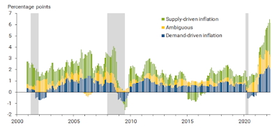
Then, armed with this categorisation, separating the overall inflation rate into the proportion coming from by demand-driven categories, and the proportion coming from supply-driven categories, is relatively straightforward. The overall picture going back to 2000 looks like this:

Notice that both sources of inflation fluctuate quite a lot, but that demand-driven inflation (the blue bars) fluctuates less than supply-driven inflation (the green bars). Note that recessions (the grey bands in the figure) tend to be characterised by demand-driven deflation (at least after the mid-point of the recession). You can also see the rapid increase in inflation in recent months, and that it has both supply-driven and demand-driven causes (as well as a large increase in ambiguous causes (the yellow bars)). However, the change in supply-driven inflation is larger than the change in demand-driven inflation. As Shapiro notes:

Supply-driven inflation is currently contributing 2.5 percentage points (pp) more than its pre-pandemic average, while demand-driven inflation is currently contributing 1.4pp more. Thus, supply-driven inflation explains a little more than half of the 4.8pp gap between current levels of year-over-year PCE inflation and its pre-pandemic average level. Demand factors explain a smaller share of elevated inflation levels, accounting for about one-third of the difference. The ambiguous category, which is not shown, explains the remainder of the difference.

It would be interesting to see whether the relative contributions of supply-driven inflation and demand-driven inflation are the same in other OECD economies, and whether differences in the drivers of inflation explain the milder inflation being experienced in some countries, when compared with others.

[HT: Marginal Revolution]

*****

[*] Which brings me to one of my pet hates. Inflation does not cause increases in prices. Inflation is a summary measure of price changes across the economy as a whole, not a driver of price changes.

[**] Increases in market power could also cause increases in prices in particular markets. However, it is unlikely that market power would increase sufficiently and simultaneously in enough markets to have an appreciable effect on inflation, despite anything you may have read. Although, market power might exacerbate changes in the inflation rate.

Your difficult-to-pronounce name could hold you back in the labour market

Both of my children have common first names. Their mother was in favour of weird names, but my feeling was that giving your child an unusual name consigned them to a lifetime of having to spell their name for people, or having to deal with mispronunciations of their name. My preference for common names was based purely on reducing the direct costs to my children, and not on how it might affect their labour market outcomes.

However, I have probably underestimated the negative impacts of having difficult-to-pronounce names. This recent working paper by Qi Ge (Vassar College) and Stephen Wu (Hamilton College) shows some significant negative effects, in the form of labour market discrimination. And those effects are independent of ethnicity. Ge and Wu note that:

Although many ethnic sounding names are also difficult to pronounce, particularly for those outside of that particular racial or ethnic group, there is still variation in the fluency of names within particular groups. For example, most non-Chinese speakers would consider Chen to be more familiar and easier to pronounce than Xiang; people without a Polish background will generally have much more trouble trying to pronounce the surname Przybylko than they will with Nowak.

Even after controlling for the ethnic or racial origin of one’s name, there are a few reasons that individuals with hard-to-pronounce names may experience worse outcomes in the labor market. There may be subconscious bias against those with difficult-to-pronounce names, leading potential employers to have more negative evaluations for these applicants and be more critical of their profiles. Recruiters will also have an easier time processing and remembering names that are more fluent and/or familiar sounding. Some individuals on hiring committees may undertake the mental effort to remember difficult sounding names, but others may not.

Ge and Wu conduct three analyses to demonstrate the labour market effects of name fluency (how easy a name is to pronounce). First:

...we utilize observational data from the academic labor market by assembling curriculum vitae (CV’s) of over 1, 500 economics job market candidates from 96 top ranked economics PhD programs from the 2016-2017 and 2017-2018 job market cycles and find that name fluency is significantly related to job market outcomes. Specifically, candidates who have difficult-to-pronounce names are much less likely to be initially placed into an academic job or obtain a tenure track position, and they are placed in jobs at institutions with lower research productivity, as ranked by the Research Papers in Economics (RePEc) database. Our results are consistent and robust across three separate ways of measuring pronunciation difficulty: an algorithmic ranking based on commonality of letter and phoneme combinations, a survey-based measure that records the average time it takes individuals to pronounce a name, and a purely subjective measure based on individual ratings.

Ge and Wu then re-analyse data from two seminal studies on labour market discrimination: (1) this 2004 study (ungated version here) by Marianne Bertrand and Sendhil Mullainathan, where the researchers sent out CVs that had either an African American name or a non-African-American name; and (2) this 2011 Canadian study (ungated version here) by Philip Oreopoulos, where CVs were sent out with Indian, Pakistani, or Chinese names, and compared with those sent out with English names. In these re-analyses, Ge and Wu find that:

In analysis of data from Bertrand and Mullainathan (2004), we find that job applicants with less fluent names have lower callback rates, even after accounting for the implied race of the candidate. What is particularly striking is the fact that within the sample of resumes with distinctly African-American names, name fluency is still strongly correlated with callback rates. We also document similar results using data from another prior audit study by Oreopoulos (2011). Once again, job applicants are less likely to be called back when they have names that are difficult to pronounce, and even when restricting the sample to immigrants with ethnically Indian, Pakistani, and Chinese names, those whose names are less fluent are significantly less likely to be called for a job interview.

Ge and Wu used three different measures of name fluency in their three analyses:

...a computer-generated algorithm that assesses the difficulty of pronouncing various words, a rating based on the median time it takes for people to pronounce a particular name, and a subjective measure based on three independent raters.

They receive similar results regardless of how they measure name fluency. Ge and Wu also explore which mechanisms may be behind the apparent discrimination, concluding that:

For job searches at academic, governmental, and research institutions, an initial screening generally involves committees getting together to discuss names of potential candidates, which may lead to some subconscious discrimination against names that are harder to pronounce and/or remember. This may also occur in the settings of prior audit studies, where recruiters must decide which applicants to call for potential interviews. Another possibility is that there are mental costs to processing and remembering less fluent names, and that these mental costs are only worth spending on higher quality candidates or when the jobs carry significant stakes. Additional analysis from both observational and experimental data seems to support this explanation. In particular, we find that PhD job market candidates with relatively weak profiles or from non-top PhD programs are more likely to suffer from name penalty in their search for academic positions. Likewise, we document similar patterns from separate analyses of Black... and Indian, Pakistani, and Chinese... applicants: those who are less qualified and have weaker resumes tend to encounter much greater discrimination due to name pronunciation than those who are more qualified and have stronger resumes.

All in all, there is some strong evidence that having difficult-to-pronounce names is negative for labour market outcomes, on top of any ethnicity-based labour market discrimination. While the study context is the US academic job market (at least for the primary analysis), it seems likely that this effect would appear more broadly across the labour market (and the secondary analyses of the two prior studies support this). It is little wonder, then, that some people choose to change their names in employment applications, as noted in a new report on Pacific workers in New Zealand prepared by the Human Rights Commission (as reported in the New Zealand Herald this week).

The solution is somehow to reduce the mental costs associated with difficult-to-pronounce names. Could that be as simple as greater exposure of people making hiring decisions to a range of different ethnic groups, or specific training in cultural intelligence, or something else? We will need some further (experimental) studies on this to find out.

[HT: Marginal Revolution]

Read more:

• What's in a (first) name?
• Uncovering labour market discrimination against foreign-born and native-born minority workers

Nobel Prize for Ben Bernanke, Douglas Diamond, and Philip Dybvig

The 2022 Sveriges Riksbank Prize in Economic Sciences in Memory of Alfred Nobel (aka Nobel Prize in Economics) was announced yesterday, with the awardees being Ben Bernanke (Brookings Institution), Douglas Diamond (University of Chicago) and Philip Dybvig (Washington University in St Louis), "for research on banks and financial crises". As usual, the award has been well covered in the media, including social media. Bernanke is the best known of the three, particularly as he was the chair of the Federal Reserve Bank at the time of the Global Financial Crisis, and responsible for the Fed's adoption of 'quantitative easing'.

Aside from Bernanke's leadership in the GFC, the three are best known for helping us to understand the role of banks in the economy. In particular, Bernanke wrote some seminal research on understanding how the unavailability of credit turned a bad recession into the Great Depression. Among other contributions, Diamond and Dybvig gave theoretical backing for the role of commercial banks in the creation of money. Their contributions are explained in more detail and very clearly in this article in The Conversation by Elena Carletti (Bocconi University):

The works by Diamond and Dybvig essentially explained why banks exist and the role they play in the economy by channelling savings from individuals into productive investments. Essentially, banks play two roles. On the one hand, they monitor borrowers within the economy. On the other, they provide liquidity to individuals, who don’t know what they will need to buy in future, and this can make them averse to depositing money in case it’s not available when they need it. Banks smooth out this aversion by providing us with the assurance that we will be able to take out our money when it’s required.

The problem is that by providing this assurance, banks are also vulnerable to crises even at times when their finances are healthy. This occurs when individual depositors worry that many other depositors are removing their money from the bank. This then gives them an incentive to remove money themselves, which can lead to a panic that causes a bank run.

Ben Bernanke fed into this by looking at bank behaviour during the great depression of the 1930s, and showed that bank runs during the depression was the decisive factor in making the crisis longer and deeper than it otherwise would have been.

Tyler Cowen at Marginal Revolution has great summaries of their contributions here (for Bernanke) and here (for Diamond and Dybvig). You can read the Nobel Committee's summary of their work here. This was a well-deserved award, and macroeconomics was due, with the last awards for macroeconomics back in 2018.

Why are students failing introductory economics?

Clark Ross (Davidson College) laments the state of students in introductory economics in this article, noting that:

...performance in my own college-level introductory economics course has been faltering. This past spring, with 31 student grades administered, I had a GPA of 2.4, essentially a flat “C.”...

Performance in the course was measured with traditional testing, particularly a very comprehensive final exam. This exam, nearly identical in both questions and content to that of prior years, had 15 multiple-choice questions covering the range of introductory economics and six short-essay questions that used more precise analysis and graphing.

The student average on the exam this past spring was just below 50 percent.

 Ross, then posits five factors that have contributed to this poor performance:

First, attendance was sporadic with many of my students. They have been told not to attend class “if they are not feeling well,” and many take that warning quite literally. For instance, on the day I introduced aggregate demand and aggregate supply, having warned students how important the lecture was, I still had nearly one-third of the students absent...

Second, work outside of class was not done with consistency. The highest-achieving student was an international student for whom English was not the first language. Yet he wrote me regularly requesting specific topics and textbook pages to prepare for class. When I asked him about it, he indicated how much easier it was for him to understand the lectures if he read material in advance of class, which he rarely missed. He admitted that his friends rarely read or studied outside of class: Economic theory seemingly did not capture their interest in the same way that reading in the humanities might. Had such students regularly attended my lectures, the absence of outside preparation would have been less damaging to them. Yet missing class and not working outside of it became a fatal combination for nearly a third of the students.

Third, basic mathematics proficiency, whatever the claims of our admissions office, is greatly lacking. This observation is relatively universal among professors in the United States today. Setting up and solving simple equations, like those needed for elasticity calculations, is truly baffling to many students...

Fourth, students seemed reluctant to come to the office seeking help. They also failed to use with great frequency the able and congenial peer tutor assigned to the course. I suspect there is an increased factor of intimidation associated with being lost in the material and asking a much older male professor for help.

Fifth, and finally, the introductory economics course... has remained somewhat constant. As a result, the student experience increasingly diverges from that of other courses, in which students feel a higher level of comfort, receive greater affirmation of their opinions, and earn higher grades. There is still a large lecture component in my course that seems dry and “outdated” to students. The traditional testing that occurs is also different from their other experiences. I fear that Economics 101 is increasingly an unpleasant outlier.

I'd say that it's likely that Ross' five factors are common to introductory economics across all of higher education, but to varying degrees. Low in-class attendance (even counting students on the live webcast) has been a particular source of frustration for me this trimester. Even having told students that attendance was a key contributor to their success (or otherwise), my ECONS101 class attendance has hovered around one-third for much of this trimester (but a lot higher in ECONS102, which is taken predominantly by economics majors). The predictable result: in the latest major assessment (with a similar format to Ross' exam), the average percentage grade for students who have been regularly attending class was 75 percent, while the average percentage grade for students not attending at all was a bit under 43 percent (and the latter is likely inflated by students who attended via webcast and did comparatively well, compared to those neither attending in-person or virtually). That isn't so different from past years, but the problem is that the proportion of students in the latter group (those not attending) has grown markedly (and despite warnings given at the start of the trimester).

Getting students to complete readings has been a challenge for a long time, but as Ross notes, it doubles down on the negative impacts on grades if students do not attend class and do not do readings. In a well-designed paper, those activities are complementary, so some learning is lost when students miss one or the other (or, increasingly, both). In some papers, students could to some extent compensate for not attending by reading more, but they are not doing that either. And when students are struggling, they are often not even seeking the help that is available. Office hours have been a bit of a joke for some time, in my experience. I could count on one hand the number of students who visit me in office hours in any given trimester. However, in my classes there are now so many ways to get help (including by reading this blog), it is difficult to say whether those other avenues are simply being used more often. Maths ability is problematic, but that factor is a problem for all subjects, not just or even specifically for economics.

All of those first four factors seem to pin a lot of the culpability for student performance on the behaviour of the students themselves. To some extent, that may be unfair, as there are things that lecturers can adjust to encourage attendance and engagement. However, the responsibility for Ross' fifth factor falls squarely on lecturers, and may be the most difficult to address. Ross provides some suggestions:

1. Explain very clearly to students, perhaps with the help of an older economics major, how to succeed in the course.
2. Give students more practice at doing problems and redoing them so they better succeed.
3. Find a way to be more welcoming and less intimidating to students seeking additional individual help.
4. Do a better job of explaining to students the relative importance of the technical material that must be applied to solve economic problems.

Or perhaps, just make lectures a bit more interactive generally? However, all of that might not be enough, when grade inflation is getting out of control. When professors are being fired (possibly paywalled for you) because their students think the class is too hard, that suggests that universities are starting to lose sight of the purpose of education, which is to have students learn something useful, not simply tick a box on their transcript. This is a point that I will return to in a future post.

[HT: Marginal Revolution for the Ross article, and Eric Crampton at Offsetting Behaviour for the NY Times article linked at the end of this post]

Fiscal drag as a cost of inflation

In my ECONS101 class, we cover the costs of inflation (albeit in the part of the paper taught by Les Oxley). One of the costs of inflation is 'tax distortions', which arises from 'bracket creep'. Apparently, bracket creep can also be referred to as 'fiscal drag'. At least, that is how it is referred to in this recent article in The Conversation, by Jonathan Barrett (Victoria University of Wellington). Barrett explains that:

New Zealand’s income tax system uses progressive rates. Higher slices of income are taxed at higher rates. Every dollar earned up to NZ$14,000 is taxed at 10.5%. Income above that level is progressively taxed higher until the final tax rate of 39% applies to every dollar earned over $180,000.

“Fiscal drag”, sometimes known as “bracket creep”, occurs when an increase in a taxpayer’s income takes their highest slice of income into a higher tax bracket without an increase in real income. This often happens when wages rise to compensate for inflation but tax bands are not adjusted.

Since it is marginal tax rates that matter for incentives, shifting taxpayers into tax brackets with higher marginal tax rates may change their behaviour, without changing their underlying real income. For example, taxpayers may choose to work more (or work less) as a result of moving into a higher tax bracket, than they would have if the brackets had adjusted along with their incomes (and wage inflation), leaving them in the same tax bracket as before. That creates unnecessary distortions in taxpayers' labour market behaviour.

Aside from lower inflation (which would decrease all of the various costs associated with inflation), the solution to fiscal drag is to adjust tax brackets for inflation, otherwise known as 'indexing'. However, it is difficult to get any taxpayer excited about the prospect of indexing tax thresholds. As Barrett notes:

Why do many employees not seem to care about fiscal drag? Perhaps it’s because, psychologically, it doesn’t feel the same as an overt tax increase. Even if the real value of your pay decreases, the amount you take home is stable.

Conversely, index linking may not feel like a tax cut. People understand that prices are rising but they may not necessarily link inflation to their tax levels.

So, unlike some of the other costs of inflation, such as menu costs and shoe leather costs, the costs of tax distortions are a bit less visible to people. In fact, these costs will be almost totally invisible to those who don't change tax brackets. That makes it difficult to convince taxpayers that policy action is necessary. Nevertheless, this is something that warrants greater attention, given that the median weekly earnings of $1189 (for wage and salary earners) is already fairly close to the $70,000 threshold ($1346 weekly) for the 33 percent marginal tax rate. It won't be too long before more than half of salary and wage earners are in that tax bracket, which would seem unnecessary given that their real incomes are not rising.

How CO2 will inflate the price of beer

The New Zealand Herald reported this week:

A lack of CO2 supply nation-wide has brewers fearful of a beer shortage this summer.

The closure of the Marsden Point refinery at the end of March means the only remaining domestic source of liquid and other food-grade CO2 is Todd Energy's Kapuni gas field in Taranaki.

Garage Project co-founder Jos Ruffell said the CO2 shortage was crippling the beverage industry.

The brewery is currently operating at 50 per cent capacity and often goes weeks at a time without being able to package beer.

What happens when there is a shortage of CO2? We'd expect the price of CO2 to rise. This is demonstrated in the diagram below, of the market for food-grade CO2. At the current market price of P0, the quantity of CO2 demanded is QD, while the quantity supplied is QS. Since QD is greater than QS, there is a shortage. When there is a shortage, some buyers are missing out. If you are a buyer in this market, how do you avoid being one of the buyers who misses out? You find yourself a seller, and you make a deal - you pay them a little bit above the market price, and they make sure that you don't miss out. In other words, when there is a shortage, buyers tend to bid the price up. This will continue until the price is bid up to P1, where the quantity demanded and the quantity supplied are both equal to Q1. At that point, the market is in equilibrium.

What does that mean for the beer market? A higher price of food-grade CO2 means that the cost of producing beer will rise. The effect of this is shown in the diagram below. The increasing cost of production decreases the supply of beer from S0 to S1. Now, if the price of beer remained at the original equilibrium price of P0, the quantity of beer demanded would remain at the original equilibrium quantity of Q0, but the quantity of beer supplied would fall to QS, creating a shortage (that is what the quote from the article above suggests). However, it seems to me that it is more likely that the price of beer will rise, to the new equilibrium price of P1.

So, you can probably expect your beer to cost a bit more this summer, thanks to the shortage of food-grade CO2.

How academic writing has changed over time

Many years ago, in a bout of enthusiasm, I read several classic novels. I coped all right with Mary Shelley's Frankenstein, and Bram Stoker's Dracula (both written in the 19th Century), but I found both James Fenimore Cooper's Last of the Mohicans and Jonathan Swift's Gulliver's Travels (both written in the 17th Century) to be heavy going. It was the language, and adjusting to the unusual turn of phrase was a challenge. In more recent times, I have had occasion to read parts of some of the classics in economics, including bits of Adam Smith's Wealth of Nations. I found that when I stray from the parts of the book that are already well known to me, it is quite taxing to read.

The challenge in these cases is the language. It is a truism that language has changed over time, and those brought up on contemporary writing can find it challenging (as I do) to read things that were written well before their time. Is that because more recent writing is easier to read in terms of word use, or because the structure, turns of phrase, and writing styles are more familiar? Based on my experiences, I suspect the latter (although I'm not convinced that they are genuinely separable, and of course there could be many other factors at play). Some mild support of my suspicions is available in this recent article by Ju Wen (Chongqing University) and Lei Lei (Shanghai International Studies University), published in the journal Scientometrics (sorry, I don't see an ungated version online). Wen and Lei look at the rate of use of adjectives and adverbs in the abstracts of journal articles published in general, biomedical and life sciences over the period from 1969 to 2019 (over 775,000 abstracts are included). They reason that, based on past research:

...adjectives and adverbs cluttered scientific writing and made scientific papers less readable...

So, greater use of adjectives and adverbs would suggest that abstracts have become less readable over time. Wen and Lei find:

...an upward trend in the use of adjectives and adverbs in scientific writing, that is, researchers used an increasing number of adjectives and adverbs in reporting their scientific findings.

And interestingly:

...the use of emotion adjectives and adverbs demonstrated a similar upward trajectory while those of the nonemotion adjectives and adverbs did not.

Of course, their analysis is mostly descriptive and doesn't actually demonstrate reduced readability, and neither does it identify why it is that the language used in abstracts has changed over time. Wen and Lei offer a couple of speculations:

To get their works published in academic journals, scientific writers may resort to linguistic devices such as emotion words (adjectives and adverbs in our case) to make their articles more positive and seemingly more appealing to editors and reviewers...

The structured abstracts usually follow an Introduction-Method-Results-Discussion format which requires the writers to summarize precisely the core information of their manuscript within a limited number of words. In such conditions, writers may become increasingly dependent on the use of adjectives and adverbs to highlight their stance and evaluation... in the study. Hence, the use of adjectives and adverbs helps writers make compelling arguments and helps readers remember key points in the full text of an article.

It would take some more detailed work, perhaps making use of exogenous changes in abstract structure or changes in editorial teams, to tease out whether either of those mechanisms explains the underlying changes. Nevertheless, if we take these results at face value, they do suggest that academic writing (at least in the sciences) is not becoming easier to read over time. So, perhaps I should persevere with the economics classics, for some time yet.

[HT: Marginal Revolution]

Book review: Spending Time

Lesson one of economics tells us that resources are scarce. For every resource, there isn't enough to do all of the things that we might want to do with it. So, we have to make choices about how best to use our scarce resources to achieve our goals. It is tempting to focus any discussion of resources on tangible resources like money (financial capital). However, doing so potentially misses the most fundamental of all resources available to us: time.

Daniel Hamermesh's 2019 book Spending Time is devoted to helping us to better understand this key resource. The book is mostly devoted to describing our current uses of time, based mainly on data from the American Time Use Survey, with occasional data from other countries including the UK, France, Germany, and Australia. The limited selection of data sources demonstrates a need for much more attention to be paid to time use. For example, New Zealand's most recent national time use survey was in 2009-10, and I believe there was only one other survey before that, in 1998-99. In one of the few times New Zealand appears in the book, Hamermesh uses data from the earlier time use survey, showing that total work (including both paid work and household production) is equal for men and women. This is a somewhat surprising fact, when set alongside other OECD countries where total work is mostly higher for women than for men. The book reveals many other surprising facts, including that:

People who are married or cohabiting state that they sleep fourteen minutes less per night than singles of the same age. 

Hamermesh focuses on four categories of time use: (1) work for pay; (2) home production ("activities that we could pay others to do for us", like cooking or cleaning); (3) personal care ("activities that are human biological necessities, such as sleeping eating or having sex"); and (4) leisure ("anything that we typically do not have to do, that we enjoy, and that we cannot outsource"). Hamermesh works through each of those categories of time use, and then presents a number of comparisons, between women and men, between young and old, between richer and poorer, and between different US regions.

I found most of the book to be somewhat unsurprising, although not always (as the quote above highlights). I also learned a number of interesting new facts (new to me, at least), including that the US has no legal mandate for paid vacations (which explains why Americans spend more hours annually in paid work than people in other countries).

The reliance mostly on a single data source, and the general nature of the topic, could easily lead to a relatively dry and lifeless book. However, Hamermesh manages to keep it interesting with anecdotes from his own experience, and the occasional humorous quip, such as:

While most vegetables are not gendered, the American couch potato is male.

I felt that the one thing that was missing from the book was a good discussion of the implications of time use. Hamermesh devotes the final chapter to this topic, but it felt a bit too much like a late tack-on to an otherwise interesting book. Given the topic, I really wanted to know how we should be spending our time better. If time is becoming more scarce (an argument Hamermesh puts forward early in the book), then what is to be done about it? The solutions seemed quite banal to me (such as spreading work time more evenly across people and across people's lifetimes).

Nevertheless, I enjoy Hamermesh's research (and have referred to it several times on this blog, including his earlier book, Beauty Pays (which I reviewed here)). If you want to know more about how people spend time, the most valuable resource, this is a useful reference book to start with.

Good reason to avoid mediation analysis

Following on from yesterday's post on the problems with instrumental variables analysis, I read this post by Uri Simonsohn on the Datacolada blog about mediation analysis. Mediation analysis has always struck me as somewhat odd, and it isn't an approach that is common in economics. And fortunately so, as Simonsohn points out that the problems with mediation analysis are actually quite serious:

In mediation analysis one asks by what channel did a randomly assigned manipulation work. For example, suppose that an experiment finds that randomly assigning Calculus 101 students to have quizzes every week (X) increased their final exam grade (Y).  Mediation analysis is used to test whether this happened because quizzes led students to study more hours through the semester (M). Mediation is present if the estimated effect of X gets smaller when controlling for M...

The problem of interest to this post is that if there is any variable, besides X, that correlates with M and Y (a very likely scenario), mediation is invalid.

Notice the similarity to yesterday's post about instrumental variables analysis. However, instrumental variables analysis might still be valid in many cases, but it requires a strong theoretical basis for the exogeneity of the instrument. For mediation analysis, this problem is probably fatal for almost all applications. Simonsohn provides a very clear explanation of why, and concludes:

In general, if we do mediation analysis, it means we expect X to lead M and Y to be correlated in our experiment. If we expect that, we should expect that other factors, confounds, cause M and Y to be correlated outside our experiment.

This post explains why such correlation invalidates mediation. In other words, this post explains why, in general, we should expect mediation to be invalid.

Simonsohn also provides some good references that provide further support for the problems with mediation analysis (along with an interesting reading that strongly critiques path analysis more generally, which I will certainly follow up on in a future post). It is certainly clear (if it wasn't already) that mediation analysis should be left out of the regular statistical toolbox.

[HT: David McKenzie on the Development Impact blog]