In my ECONS101 class this week, I had to rush through the last bit of the lecture. So, I thought it might be handy to outline the last example we were working on in a bit more detail. It relates to the stylised facts outlined in the figure below, which comes from Unit 3 of The Economy (the textbook we use in ECONS101), but the original data comes from Robert Fogel's book The Fourth Great Awakening and the Future of Egalitarianism.

The figure shows the estimated lifetime hours of discretionary time (24 hours per day, minus the time spent sleeping, eating, and on personal hygiene) in blue, and breaks discretionary hours down into lifetime work hours (in red) and lifetime leisure hours (in green), for 1880, 1995, and a projection for 2040. The interesting thing here (aside from the increase in discretionary hours over time), is the big increase in leisure hours between 1880 and 1995, and reduction in work hours. That change in leisure and work happened in spite of a substantial increase in real wages over the same period.
These facts should come as a little bit of a surprise. That's because we expect that, when wages are higher, people should be working more, not less. In other words, we expect the supply of labour to be upward sloping. The reason we expect people to work more is because, as wages rise, the opportunity cost of leisure increases - every hour spent in leisure means that the worker gives up more income than before. When the opportunity cost of doing something increases, we expect people to do less of it. But in this case, as the opportunity cost of leisure has increased, workers are consuming more leisure, not less.
To understand and explain this puzzle, we need a model. In this case, it is a model of the work decision of workers. In the work decision, the worker is asked to trade off between two goods: leisure, and consumption (or income). The worker wants more leisure, but for every hour of leisure, they give up an hour of working, which means their income (and consumption) will be lower. If the worker wants higher income, they have to give up an hour of leisure.
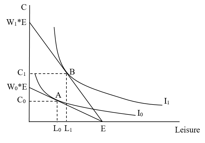
Our model of the worker's decision is outlined in the diagram below. The worker's decision is constrained by the amount of discretionary time available to them. Let's call this their time endowment, E. If they spent every hour of discretionary time on leisure, they would have E hours of leisure, but zero income. That is one end point of the worker's budget constraint, on the x-axis. The x-axis measures leisure time from left to right, but that means that it also measures work time (from right to left, because each one hour less leisure means one hour more of work). The difference between E and the number of leisure hours is the number of work hours. Next, if the worker spent every hour working, they would have zero leisure, but would have an income equal to W0*E (the wage, W0, multiplied by the whole time endowment, E). That is the other end point of the worker's budget constraint, on the y-axis. The worker's budget constraint joins up those two points, and has a slope that is equal to the wage (more correctly, it is equal to -W0, and it is negative because the budget constraint is downward sloping). The slope of the budget constraint represents the opportunity cost of leisure. Every hour the worker spends on leisure, they give up the wage of W0. Now, we represent the worker's preferences over leisure and consumption by indifference curves. The worker is trying to maximise their utility, which means that they are trying to get to the highest possible indifference curve that they can, while remaining within their budget constraint. The highest indifference curve they can reach on our diagram is I0. The worker's optimum is the bundle of leisure and consumption where their highest indifference curve meets the budget constraint. This is the bundle A, which contains leisure of L0 (and work hours equal to [E-L0]), and consumption of C0.

Now, consider what happens when the wage increases. Real wages (adjusted for inflation) increased a lot between 1880 and 1995. This is shown in the diagram below. For simplicity, let's assume that the worker's time endowment remained the same [*]. As the wage increases, the worker's budget constraint pivots outwards and becomes steeper. It has the same intercept on the y-axis x-axis (equal to the time endowment E), but if the worker spent every discretionary hour working, they would now have consumption (and income) equal to W1*E, where W1 is the new (higher) wage. Notice that the new budget constraint is steeper. This is because the slope of the budget constraint is equal to the wage, and the wage is now higher (and a higher value for the slope means a steeper line). The worker can now reach a higher indifference curve (I1). Their new optimal bundle of leisure and consumption is B, which contains leisure of L1 (and work hours equal to [E-L1]), and consumption of C1. Notice that the worker now consumes more leisure and more consumption as well. Because leisure has increased, that means that the number of work hours has decreased.
Coming back to the key facts we started this post with, the model does clearly show that, when wages go up, the worker will consume more leisure (and work less). Where did our original intuition go wrong?
Our original explanation, that as the wage increases the opportunity cost of leisure increases, and the worker will choose to work less, is the substitution effect of the change in the wage. However, when the relative price of two goods changes, the substitution effect is not the only thing that affects constrained decisions. There is also an income effect. In this case, the income effect says that, when wages go up, the worker can afford more consumption, but can also afford more leisure. Since both leisure and consumption are normal goods (we demand more as our income increases), the worker will want more leisure (and will want to work less). Over the period from 1880 to 1995, the income effect must have been larger than the substitution effect, and has driven the decrease in work hours (and increase in leisure hours).
Does this mean that increasing wages will always induce workers to work less? Of course not. The increase in real wages over the period from 1880 to 1995 was huge. And, no individual worker working in 1880 was still working in 1995, so no worker actually experienced the change we represented in our model. Most wage changes are much more modest, and it does appear that labour supply curves are generally upward sloping at the level of wages we observe over the short run. What that means is that the income effect is likely to be much smaller than what our diagram shows (and that would mean that L1 would be slightly to the left of L0. I'll leave drawing that situation as an exercise for you.
*****
[*] We know this isn't true, but it helps to make this assumption because we are more interested in the effect of the change in wages, and not the effect of the change in time endowment.
made a mistake, "It has the same intercept on the y-axis (equal to the time endowment E)". Supposed to be x-axis?
ReplyDeleteYes, you're right. It should be the x-axis. I'll make that change.
Delete