Tuesday 31 May 2022

The interesting incentive effect of reducing the drink driving limit in Utah

Many countries have lowered their breath alcohol limits for driving in recent years. New Zealand lowered the limit from 400 micrograms of alcohol per litre of breath to 250 in December 2014. The idea is (unsurprisingly) that fewer people would drive while intoxicated, leading to fewer accidents and fewer injuries and deaths. It is unclear what the effect of the change in New Zealand was (statistically, it is difficult to determine), but this new working paper by Javier Portillo (University of Louisiana at Lafayette), Wisnu Sugiarto (Washington State University), and Kevin Willardsen (Wright State University). In March 2017, Utah became the first state in the U.S. to lower the blood alcohol limit from 0.08 g/dL to 0.05 (this is equivalent to the change in breath alcohol limit that New Zealand adopted). Portillo et al. look at the effect of that change on traffic accidents, using:

...a difference-in-differences (DID) estimator on Utah counties using the counties of neighboring states - Idaho, Nevada, Colorado, and Wyoming - as controls.

Essentially, this DID strategy involves comparing the difference between two differences: (1) the difference in traffic accidents before and after the limit change for Utah counties; and (2) the difference in traffic accidents before and after the limit change for neighbouring counties outside Utah. The assumption here is that the two differences would be the same if Utah had not reduced the drink driving limit.

Portillo et al. use data collected independently from each state's Department of Transportation (presumably, there is no central data repository where appropriate data are available). They find that:

...the policy reduced the total number of traffic accidents in Utah. This drop, is primarily in property damage-only accidents in urban counties... Effects during the day are twice the size relative to those at night, and several times larger than those found on weekend nights where we would expect the largest result. Estimates suggest a reduction of approximately 74 and 34 property damage accidents, per quarter, for the median urban county for days and nights respectively, which is roughly an 8.5 and 4.0 percent reduction in total accidents.

These results seem a bit puzzling. You would expect a change in the drink driving limit to affect night-time crashes rather than day-time crashes, and to affect crashes that involve injuries, rather than property-damage-only crashes. However, Portillo et al. then discuss the incentive effects related to the law change:

A possible explanation for the observed outcome is that the policy is doing more to driver behavior than just preventing drivers with a BAC between a 0.05-0.08 from driving. The costs of a DUI in Utah are high. Driving under the influence is considered a class B misdemeanor, at the very least (and a class A misdemeanor under other circumstances)...

Keeping these costs in mind, consider the following scenario. An individual has few drinks at brunch, lunch, or early dinner and gets into an accident. If the accident involves an injury, police are notified and dispatched, they take a report, and the driver risks a DUI because she must interact with the officers. However, if the accident is property damage only, there are no legal requirements to involve police if the estimated damages are under $1,500.47 Instead of risking the DUI and its consequences, the driver takes responsibility for the accident, exchanges insurance information, and leaves. This is done because it may cheaper than a DUI in the long run. If the police never arrive, the accident is never reported; but this will only happen for property damage only accidents. The one thing that typically guarantees the arrival of police is an injury. If it is during the weekday, where we find the largest effect, individuals may also have a reason to resolve such issues with haste (or not wait for the police): work... This may explain the over representation of a fall in property damage only accidents we have identified. It is not so much that the accidents are not taking place, but that they are not being reported. This suggests that at least some of the effect found is not a reduction in total accidents, but a reduction in the reporting of property damage only accidents.

As anyone who has done any economics class should know, people respond to incentives. The change in the drink driving limit creates a stronger incentive not to drink and drive, but it also creates a stronger incentive not to report minor accidents. If minor accidents are being reported less in Utah than in other counties after the change in the drink driving limit, than that would appear to show a reduction in minor traffic accidents, as Portillo et al. find, even if the rate of more serious injury accidents does not change at all. The disappointing result here from a research perspective is that the incentive effects mean that we don't end up knowing whether the law change resulted in a reduction in motor vehicle accidents overall, or not.

[HT: Marginal Revolution]

Monday 30 May 2022

Gender differences in dropping out of university and switching majors

Some seven years ago, I had a couple of summer research scholarship students look at dropping out of university (specifically, the management degree at the University of Waikato), including the factors associated with dropping out, and what led to student persistence. One factor that strongly predicted dropping out was gender - male students had over one-third lower odds of completing their degree than female students.

So, I was interested to read this 2018 article by Carmen Astorne-Figari and Jamin Speer (both University of Memphis), published in the journal Economics Letters (sorry, I don't see an ungated version online). They specifically look at gender differences in dropping out, as well as gender differences in switching majors, at university. Using data from the 1997 cohort of the National Longitudinal Study of Youth (NLSY97), which included nearly 3000 students who attended college and reported at least one GPA, Astorne-Figari and Speer found that:

Males are 7.7 percentage points (or 22%) more likely to drop out. The male-female differential is about the same as the effect of one point of GPA... the gender gap reverses for major switching: women are 7.6 percentage points more likely than men to switch majors. These effects perfectly offset so that there is no gender gap in major persistence. This is in contrast to the racial/ethnic gaps, as both blacks and Hispanics are more likely to drop out and to switch majors.

So, the higher dropout rate for male students that my summer students found is not an aberration. Male students do appear to drop out in significantly greater numbers than female students do. However, the rate of completion of the major that students started their studies in does not differ between male and female students. One way of interpreting these results is that it appears that male and female students respond differently to the challenges of university study. If they find themselves in a field of study that they are not enjoying or doing well in, male students respond by dropping out, while female students respond by switching majors. Of course, it would be interesting to stratify the analysis by GPA, and see if there are really differences for students at the bottom end of the GPA distribution, but Astorne-Figari and Speer don't do that. However, they do look in more detail at STEM subjects and, interestingly, the results are slightly different:

Again, men are more likely to drop out of college, while women are more likely to switch out. Both gaps here are larger than in the overall sample, and the switching gap is particularly large... Women are 19.9 percentage points more likely to switch out of STEM, doubling the switching rate of men.

Unlike the overall results, there is a substantial gender gap in persistence for those who start in STEM fields. Women are 7.9 percentage points (18%) less likely to graduate in a STEM major conditional on starting one, driven by the huge gap in switching behavior.

So, completion rates of STEM majors are lower among female students than among male students. That may help to explain some of the gender gap in STEM graduates. However, it also poses a bit of a dilemma. Ideally, universities want to reduce the rate of students dropping out. But, if they implement some policy intervention to reduce dropout rates, more male than female students might be affected (if only because there are more male dropouts). That would tend to increase the gender gap in STEM even further, a point that Astorne-Figari and Speer also note:

...men’s higher dropout rates are actually keeping the STEM gender gap from being even larger, so better retention might also widen the gender gap in STEM.

However, one way of addressing disparities in dropout rates while not exacerbating the STEM gender gap might be to try policy interventions that help male students to change majors, rather than dropping out. Perhaps there is some other field that they are better suited to, but for some reason female students are better able (or more willing) to identify a new field than male students. This seems like something worth further investigation. 

Sunday 29 May 2022

Migration and working age population decline in Europe

It is more than simply a truism to say that populations are ageing over time. Structural ageing (changes in the age distribution of the population, whereby older people constitute a larger proportion of the total population) is a real phenomenon, observed across all countries and regions of the world. However, the areas worst affected by structural ageing tend to be remote regions, where young people are out-migrating to cities in large numbers.

One way that structural ageing can manifest is in the size of the working age population (this can be defined in various ways, but a common approach is the population aged 15-64 years). As the population ages, a larger proportion of the population is aged 65 years or over (and no longer in the working age population), and so the working age population shrinks. Similarly, as young people migrate out of a country or region, the working age population shrinks.

So, I was interested in this recent article by Daniela Ghio, Anne Goujon, and Fabrizio Natale (all European Commission Joint Research Centre), published in the journal Demographic Research (open access, with a shorter non-technical summary available on N-IUSSP). They look at to what extent cohort turnover and migration effects affect the size of the working age population for regions across the European Union countries (specifically, for NUTS3 regions - the smallest disaggregation of regions used by Eurostat) over the period from 2015 to 2019. Cohort turnover is specified as the difference between the size of the cohort of young people at labour market entry age (15-19 years) and the size of the cohort of older people at labour market exit age (60-64 years). Migration is the net migration of the working age population. Comparing those two values with change in the working age population over the period, Ghio et al. categorise four different types of regions. The first type of region was:

NUTS3 territorial units where both components are positive represented approximately 8% of territories (13% of EU working-age population in 2019), mainly distributed across the following countries: the Netherlands (20 territories), Belgium (15), Spain (12), and Germany (11).

In the vast majority of territories (94), the positive effects coincided with an increase in the size of the working-age population during the 2015–2019 period...

Next:

The cluster with positive cohort turnover effects and negative net migration was the smallest one: only 5% of EU territories accounting for 11% of the EU working-age population in 2019, mostly located in France (30). Among these, the majority (54 territories, corresponding to 8% of the EU working-age population) reported a decrease in the size of the working-age population.

Third up: 

The cluster with negative cohort turnover effects and positive net migration included the largest share (63%) and number (738) of EU territories, representing 54% of the EU working-age population in 2019.

Finally:

The cluster with both negative cohort turnover effects and net migration was the second largest and consisted of 266 territories, corresponding to 23% of EU territories and 22% of the EU working-age population in 2019, mostly distributed across eastern EU MS such as Bulgaria (18), Romania (31), and Hungary (9); central eastern EU MS such as Poland (40); south-eastern EU MS such as Croatia (18); and southern EU MS such as Greece (18) and Italy (41).

The four types of region are nicely illustrated in Figure 2 from the paper:

The overall decline in the size of the working age population is readily apparent in the first panel of the figure, on the left. Notice that much of that change is due to population ageing (the cohort turnover in the third panel, on the right) rather than net migration (the middle panel). I suspect this would be a general feature not just for Europe, but for all western countries, including New Zealand and Australia.

This is a nice paper, which offers an interesting characterisation of regions across two dimensions: (1) whether cohort change is increasing or decreasing the size of the working age population; and (2) whether net migration is increasing or decreasing the size of the working age population. I have done similar analyses in the past (unpublished as yet), but also looking dynamically as to how the changes in components (in my case, it was natural increase or decrease [births minus deaths] and net migration) move over time. This is the sort of analysis that local planners and policy makers are really interested in. Importantly, it doesn't require much in the way of data or heavy analytical skills. It would be really interesting to see a similar analysis for New Zealand - a good potential project for a future Honours or Masters student.

[HT: N-IUSSP]

Wednesday 25 May 2022

Husbands vs. wives

On the Development Impact blog back in March, Markus Goldstein pointed to this fascinating NBER Working Paper by John Conlon (Harvard University) and co-authors, innocuously titled "Learning in the Household". Despite the title, the working paper reveals a study of how husbands and wives treat information revealed by each other differently (a finding that will no doubt come as no surprise to my wife).

Conlon et al. recruited 400 married couples and 500 unrelated strangers (with equal numbers of men and women) for their study, in Chennai (India) in 2019. In the experiment, research participants:

...play five rounds - with different treatments - of a balls-and-urns task... The goal in each round is to guess the number of red balls in an urn containing 20 red and white balls. Participants are informed that the number of red balls is drawn uniformly from 4 to 16 in each round...

In each round, participants receive independent signals about the composition of the urn. Concretely, they privately draw balls from the urn with replacement. Depending on the round, they either play the game entirely on their own or else can learn some of the signals from their teammate. Comparing learning across these rounds allows us to test for frictions in communication and information-processing which may interfere with social learning.

Seems straightforward so far. The experiment involves several rounds, which proceed somewhat differently from each other:

Individual round. The Individual round proceeds as follows. First, the participant draws a set of balls from the urn, followed by a guess of how many red balls are in the urn. Then, they draw a second set of balls from the urn and make a second (and final) guess. All drawing and guessing is done privately, without any opportunity to share information. This round serves as a control condition - a benchmark against which we compare the other conditions.

Discussion round. The Discussion round differs from the Individual round in that, for each participant, their teammate’s draws - accessible through a discussion - serve as their ‘second’ set of draws. Each person first makes one set of draws followed by a private guess, exactly as in the Individual round. Next, the couple are asked to hold a face-to-face discussion and decide on a joint guess. After their discussion and joint guess, each person makes one final, private guess.

By comparing the final private guesses in the individual round and the discussion round, Conlon et al. can test whether learning your teammate’s information through a discussion is just as good as receiving the information directly yourself. There are two further rounds as well:

Draw-sharing round. This round is identical to the Discussion round except that, after participants receive their first set of draws and enter their first guess, they are told their teammate’s draws (both number and composition) directly by the experimenter, e.g. “Your spouse had five draws, of which three were red and two were white.” They then make an additional private guess which can incorporate both sets of draws before moving on to the discussion, joint guess and final private guess...

Guess-sharing round. The Guess-sharing round is the same as the Draw-sharing round except that the experimenter informs each person of their spouse’s private guess (made based on their own draws only), rather than their spouse’s draws. The experimenter also shares the number of draws this guess was based on, e.g. “Your spouse had 5 draws and, after seeing these draws, they guessed that the urn contains 12 red balls.”

By comparing the final private guesses in the individual round and the draw-sharing round, Conlon et al. can test whether the identity of who learns the information matters (aside from who shares that information). By comparing the final private guesses in the discussion round and the draw-sharing round, Conlon et al. can test the extent to which communication frictions affect decision-making (since there are no frictions in the draw-sharing round, because the information is shared by the experimenter, and the teammates cannot discuss at all). Comparing the draw-sharing round and the guess-sharing round allows Conlon et al. to test whether beliefs about the competence of the teammate matters. Finally, having teams made up of spouses or made up of mixed-gender strangers or same-gender strangers allows Conlon et al. to see if spouses share information (or act on information) differently than strangers do.

Having run these experiments, Conlon et al.:

...first compare guesses in the Individual and Discussion rounds, played in randomized order. Husbands put 58 percent less weight (p<0.01) on information their wives gathered - available to them via discussion - than on information they gathered themselves. In contrast, wives barely discount their husband’s information (by 7 percent), and we cannot reject that wives treat their husband’s information like their own (p=0.61). The difference in husbands’ and wives’ discounting of each other’s information is statistically significant (p=0.02).

The lower weight husbands place on their wives’ information is not due of a lack of communication from wives to husbands. In another experimental treatment - the Draw-sharing round - husbands put less weight on their wife’s information even when it is directly conveyed to them by the experimenter (absent any discussion). In this case, husbands discount information collected by their wives by a striking 98 percent compared to information collected by themselves (p<0.01), while wives again treat their spouses’ information nearly identically to their own. Lack of communication between spouses or husbands’ mistrust of (say) wives’ memory or ability thus cannot explain husbands’ behavior. Rather, husbands treat information their wives gathered as innately less informative than information they gathered themselves. In contrast, wives treat their own and their husbands’ information equally.

The guess-sharing round doesn't appear to reveal too much of interest, with results that are similar to the draw-sharing round. Finally, comparing the results from teams of spouses with the results from teams of strangers, Conlon et al. find that:

In both mixed- and same-gender pairs, men and women both respond more strongly to their own information than to their teammate’s. Thus, the underweighting of others’ information appears to be a more general phenomenon. Husbands treat their wives (information) as they treat strangers; wives instead put more weight on their husband’s information than on strangers’ information.

There is a huge amount of additional information and supporting analysis in the working paper (far too much to summarise here), so I encourage you to read it if you are interested. Conlon et al. conclude that there is:

...a general tendency to underweight others’ information relative to one’s ‘own’ information, with a counteracting tendency for women to weight their husband’s information highly.

Now of course, this is just one study that begs replication in other contexts with other samples. However, I'm sure there is a large section of the population who would find that conclusion meets their expectations (and/or their lived experience).

[HT: Markus Goldstein at Development Impact]

Sunday 22 May 2022

The global inequality boomerang

Overall, global inequality has been decreasing over the last several decades. That may contrast with the rhetoric about inequality that you are familiar with from the media. However, the global decrease in inequality has mostly been driven by the substantial rise in incomes in China. However, China's contribution to decreasing global inequality may be about to change. In a new working paper, Ravi Kanbur (Cornell University), Eduardo Ortiz-Juarez and Andy Sumner (both King’s College London), discuss the possibility of a 'global inequality boomerang'.

Focusing on between-country inequality (essentially assuming that within-country inequality doesn't change), and using a cool dataset on the income distribution for every country scraped as percentiles from the World Bank's PovcalNet database, Kanbur et al. find that:

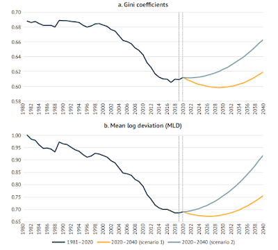
...there will be a reversal, or ‘boomerang’, in the recent declining (between-country) inequality trend by the early-2030s. Specifically, if each country’s income bins grow at the average annual rate observed over 1990–2019 (scenario 1), the declining trend recorded since 2000 would reach a minimum by the end-2020s, followed by the emergence of a global income inequality boomerang...

This outcome is illustrated in their Figure 4, which shows the historical decline in inequality since the 1980s, along with their projections forward to 2040:

Scenario 1 assumes an almost immediate return to pre-pandemic rates of growth. Scenario 2 assumes slower growth rates for countries with lower rates of vaccination. Neither scenario is particularly likely, but the future trend in global inequality is likely to be somewhere between them, and likely to be moving upwards. Why is that? Between-country inequality has been decreasing as China's average income has increased towards the global average. In other words, Chinese household incomes have increased, decreasing the gap between Chinese households and households in the developed world. However, once China crosses the global average, further increases in Chinese average income will tend to increase between-country inequality.

Of course, this might be a pessimistic take, because if other populous poor countries (including India, Indonesia, Pakistan, Nigeria, and Ethiopia) grow more quickly, then their growth might reduce inequality enough to offset the inequality-increasing effect of Chinese growth. However, that is a big 'if'. According to World Bank data, China's GDP per capita growth rate averaged 8.5 percent per year between 1991 and 2020. Compare that with 4.2 percent for India, 3.2 percent for Indonesia, 1.5 percent for Pakistan, 1.4 percent for Nigeria, and 3.9 percent for Ethiopia. These other countries would have to increase their growth rates massively to offset Chinese growth's effect on inequality.

This isn't the first time that Chinese growth has been a concern for the future of global inequality. Branko Milanovic estimated back in 2016 that China would be contributing to increasing global inequality by 2020 (see my post on that here). Things may not have moved quite that quickly (a pandemic intervened, after all). Kanbur et al. are estimating under their Scenario 1 that the turning point will be around 2029 (and around 2024 under their Scenario 2). Slower Chinese growth, and faster growth in the rest of the world, have no doubt played a part in this delay. However, it's likely that the turning point in global inequality cannot continue to be delayed for much longer.

Read more:

Saturday 21 May 2022

Ian Pool, 1936-2022

I was very saddened to hear of the passing of Ian Pool at the end of last month. I have held off on posting about this, waiting for a good obituary to show up online. I was not to be disappointed - Stuff published a beautiful obituary by Brian Easton earlier today. For those who don't know, Ian Pool is widely regarded as the founding father of New Zealand demography. He set up the Population Studies Centre (PSC) at the University of Waikato, which remains a national centre of excellence in demography and population studies (in its latest incarnation, renamed as Te Ngira - Institute for Population Research). Ian was well known for his work on African demography, as well as Māori demography, among many other contributions to the field.

I had many interactions with Ian over the years, including as a co-author and a co-researcher. When I first met him, sometime in the mid-2000s, I was working as a research assistant for Jacques Poot at the PSC, and completing my PhD in economics. Ian initially struck me as one of those infuriating people who have the habit of constantly name-dropping famous people they have met. However, Ian's name-dropping wasn't merely a cynical attempt to big-note himself - he really did know and had closely interacted with Joseph Stiglitz, Thomas Piketty, and others. And I have to admit feeling a bit of a warm glow some years later when Ian name-checked me in a seminar or presentation (more than once) for my work on stochastic population projections.

My interactions with Ian also resulted in what is possibly one of the big missed opportunities of my career. Ian was very keen to have me work on a new research idea, distributional national accounts. I was mildly interested, but didn't have the time to devote to it immediately. I also had other priorities, especially in trying to establish a longitudinal ageing study based at Waikato (an initiative that eventually proved to be a dead end, as despite a lot of positive end-user engagement, we couldn't secure sufficient funding to make the study feasible). Anyway, I hadn't realised at the time just how important the idea of distributional national accounts was to become, as well as its centrality to the work of Piketty, Emmanuel Saez, and others. Distributional national accounts were also a key contribution to the work of the High-Level Expert Group on the Measurement of Economic Performance and Social Progress, co-chaired by Stiglitz, Fitoussi, and Durand, as noted in the book Measuring What Counts (which I reviewed here). Ian was at the cutting edge, but sadly, I don't believe that he did find someone to work on New Zealand's distributional national accounts.

I was never a student of Ian's, but I did sit in on a workshop that he gave some years ago, on how to derive and interpret life tables. He was an excellent communicator, and clearly would have been a great teacher and mentor to students at all levels. I have had the pleasure of working with a number of his excellent former PhD and graduate students, including Natalie Jackson and Tahu Kukutai. I'm sure that a more complete roll call of Ian's students would reveal just how much of an impact he has had, and continues to have, on population studies and demography both in New Zealand and internationally.

Aside from his research contributions, Ian was just a lovely, generous, and sincere man. He was patient and kind to colleagues and students alike, and a fountain of knowledge on many things. He will be greatly missed.

Friday 20 May 2022

The problem with studies on the relationship between alcohol outlets and sexually transmitted diseases

I've done a fair amount of research on the impacts of alcohol outlets on various measures of alcohol-related harm. That work has focused predominantly on violence, property damage, and crime generally. One thing I haven't looked at is the relationship with sexually transmitted diseases. That is for good reason. Crime is an acute outcome associated with drinking, and is measurable almost immediately. That distinguished crime from longer-term negative consequences of drinking such as liver cirrhosis, for example.

However, in-between those two extremes are some alcohol-related harms that we could refer to as medium-term harms. For example, the theoretical link between alcohol consumption and risky behaviour, including risky sex, seems clear. So, if having more alcohol outlets in a particular area is associated with greater alcohol consumption (following availability theory, as I discussed in this post earlier this week), then alcohol outlets should be positively associated with greater prevalence of sexually transmitted diseases. Sexually transmitted diseases do not become immediately apparent in the way that violence or property damage does, but they don't take years to manifest in the way that cirrhosis does.

There have only been a few studies on the relationship between alcohol outlets and sexually transmitted diseases. So, I was interested to read two studies recently related to this topic, which had been sitting on my to-be-read pile for some time. The first study was reported in this 2015 article by Molly Rosenberg (Harvard School of Public Health) and co-authors, published in the journal Sexually Transmitted Diseases (ungated NLM version here). They look at the relationship between alcohol outlets and Herpes Simplex Virus Type 2 (HSV-2) prevalence among young women (aged 13-21 years) in the Agincourt Health and Demographic Surveillance System site in South Africa. The Agincourt sample has predominantly been used as an HIV surveillance site, and there are dozens of studies based on this sample. However, they didn't look at HIV as an outcome in this study:

...because of the small number of prevalent infections at baseline and the likelihood that at least some of the cases were a result of perinatal, as opposed to sexual, transmission.

Fair enough. Perinatal transmission of HIV (transmission at or around the time of birth) has been a serious problem, but I guess it must be less of a problem for HSV-2. In their analysis, Rosenberg et al. essentially counted the number of alcohol outlets (both on-licence and off-licence combined) in each village, and related that number to HSV-2 prevalence for the 2533 young women in their sample. They found that:

Treating the alcohol outlet exposure numerically, for every 1-unit increase in number of alcohol outlets per village, the odds of prevalent HSV-2 infection increased 8% (odds ratio [OR; 95% CI], 1.08 (1.01–1.15]). The point estimate changed minimally after adjustment for village- and individual-level covariates (OR [95% CI], 1.11 (0.98–1.25]); however, this adjusted estimate was less precise.

Not only was it less precise, but it becomes statistically insignificant (barely), which they don't note. So, this doesn't provide strong evidence of a link between alcohol outlets and sexually transmitted diseases, although the evidence is suggestive. The problem is that the analysis essentially assumes that all young women in the same village have the same exposure to alcohol. This marks the number of outlets as an imperfect proxy for the real exposure variable, and suggests that the real effect might be larger. Again, this is suggestive evidence at best.

The second study was reported in this 2015 article by Matthew Rossheim (George Mason University), Dennis Thombs, and Sumihiro Suzuki (both University of North Texas), published in the journal Drug and Alcohol Dependence (sorry, I don't see an ungated version of this one online). This study did look at HIV as an outcome, relating zip-code-level HIV prevalence to the number of alcohol outlets (of different types) across 350 cities in the US. Perinatal transmission of HIV is not much of a problem in the US (certainly not compared to South Africa at the time that the Agincourt sample were born). Based on their data for a little over 1000 zip codes, Rossheim et al. found that:

...the presence of one additional on-premise alcohol outlet in a ZIP code was associated with an increase in HIV prevalence by 1.5% (rate ratio [RR] = 1.015). In contrast, more beer, wine, and liquor stores and gas stations with convenience stores were associated with lower HIV rates (RR = 0.981 and 0.990, respectively). Number of pharmacies and drug stores was not associated with HIV prevalence (p = 0.355).

On-premise outlets (predominantly bars and nightclubs) were associated with higher HIV prevalence, while liquor stores and gas stations were associated with lower HIV prevalence. Rossheim et al. don't have a good explanation for why, although they note a number of obvious limitations with their study. The literature on the impacts of alcohol outlets is littered with these sorts of inconsistent findings.

The real problem with a study like this is the time lapse between the alcohol consumption and the measured outcome variable. As I noted at the start of this post, with acute harm (like violence or property damage), the effect is immediately seen and can be measured, and likely occurred close to the location of alcohol consumption. With HIV prevalence, there is only a small chance that HIV was contracted as a result of activity within the local area. People move about over time, they 'interact' with people in many locations, and they can migrate from city to city. So, all we can say with this study is that people living with HIV tend to live in areas that have lots of bars and night clubs, and tend to live in areas that have fewer liquor stores and gas stations. Call this the gay-men-live-near-night-clubs effect, if you want to evoke a bunch of stereotypes. This effect is correlation, and it is difficult to say with any certainty if there is any causal relationship here.

Now, the Agincourt study has this problem as well, but the young women there probably still live in the same village they grew up in, so in that case the exposure to alcohol can be (imperfectly, as I noted above) proxied by the number of outlets in the village. And the symptoms of HSV-2 appear within a week, rather than weeks or months later as can be the case for HIV. So, moving about is less of an issue, although not eliminated entirely.

Anyway, these two studies are interesting, but they mainly highlight the problems with this broader literature. When we move beyond measuring acute harms associated with alcohol outlets, it isn't clear that the associations that are being measured are anything more than spurious correlation.

Thursday 19 May 2022

Stephen Hickson on the fight against woolly words

I'm loving Stephen Hickson's work lately. In addition to writing about the stupidity of removing GST from food last week (which I posted about here), and co-authoring a piece in The Conversation with myself and others on our 'quick takes' on Budget 2022, he wrote the most hilarious post on LinkedIn yesterday:

Woolly words...

I came across this article today (not sure if you need a subscription to read it or not but the gist of it is in the first paragraph "FIRE-FIGHTING FOAM starves the flames of oxygen. A handful of overused words have the same deadening effect on people’s ability to think. These are words like “innovation”, “collaboration”, “flexibility”, “purpose” and “sustainability”. They coat consultants’ websites, blanket candidates’ CVs and spray from managers’ mouths. They are anodyne to the point of being useless. These words are ubiquitous in part because they are so hard to argue against."

https://lnkd.in/dGmNY_ub

Imagine if the government becomes aware of the damage that the excessive use of these words is causing… there's a good chance that the Government will sign up to an international accord to limit the use of Woolly Words. In an attempt to make good on that commitment they will introduce a Woolly Words Trading Scheme (WWTS). In order to get political buy-in some sectors will initially be exempt despite being the biggest users of Woolly Words, e.g. Marketing companies. Additionally the cap on Woolly Words won’t initially be binding and so everyone will agree that the WWTS is pretty weak. Eventually this will get fixed though it will take a while. But a WWTS isn’t very sexy and doesn’t look like the government is really doing anything. So they’ll start doing things that make little sense and are expensive but look a lot sexier. For example they’ll offer to subsidise at great expense the use of better words in mission statements and annual reports of some arbitrarily favoured organisations in return for them reducing their own use of Woolly Words. Or they’ll simply ban the use of Woolly Words in some sectors such as health. While this makes these organisations and sectors less woolly it doesn’t reduce the overall quantity of Woolly Words available when the WWTS is binding. It couldn't possibly happen could it?

It's not hard to see that this is a satirical take on the emissions trading scheme, including the exclusion of agriculture, and the various tinkering the government undertakes to try and solve problems that would more easily be solved if the scheme were comprehensive. In my ECONS102 class, we characterise an efficient property rights system as one that has four key features:

  1. Universal - all resources are privately, publicly, or communally owned and all entitlements are completely specified;
  2. Exclusive - all benefits and costs accrued as a result of owning and using the resources should accrue to the owner whether directly or indirectly;
  3. Transferable - all property rights should be transferable from one owner to another in a voluntary exchange; and
  4. Enforceable - property rights should be secure from involuntary seizure or encroachment by others.

The emissions trading scheme (and the woolly words trading scheme) creates a property right - the right to emit carbon (or the right to use woolly words). The scheme will only be efficient if it is universal - that is, all emissions (or woolly words) must be covered by the scheme. When agriculture (or marketing) is excluded, they can generate as many emissions (or woolly words) as they like, essentially without consequence. If the government is concerned about their emissions (or woolly words), then the government has to create all sort of other regulations to keep them in line. Which is completely unnecessary, since including them within the trading scheme would be much more efficient (lower cost, and simpler all around).

If we really are concerned about carbon emissions (or woolly words), we have the means to limit them. Excluding favoured sectors from the trading scheme is pure politics, combined with a fair amount of fingers-in-the-ears-I'm-not-listening-to-you, and that is going to cost us far more in the long term.

Tuesday 17 May 2022

Fast food outlets, obesity, and why we do meta-analysis

Some time back, someone (I forget who) pointed me to this report by Christopher Snowdon (Institute of Economic Affairs) on the relationship between the density of fast food outlets and obesity. It was of interest to me because the underlying theory linking fast food outlets to obesity is substantively the same as one of the key theories linking alcohol outlets and various measures of alcohol-related harm. That theory is known as availability theory, and posits that more outlets (fast food, or alcohol) in a particular area reduces the 'full cost' of the good (fast food, or alcohol), and therefore increases consumption (the straightforward consequence of a downward-sloping demand curve). The 'full cost' includes the price, as well as the cost of travelling to obtain the good. Both of those components of the full cost may be lower when there are more outlets. Price may be lower due to greater local competition, while travel cost may be lower because each consumer will likely live closer to the nearest outlet. The last component of availability theory is that because there is more consumption (fast food, or alcohol), there are more problems (obesity, or alcohol-related harms). This last component is essentially taken on faith.

Anyway, Snowdon summarises the literature analysing the relationship between fast food outlets and obesity, which is made up of 74 studies published between 2004 and 2017. I say summarise, rather than review, for good reason. Snowdon's report doesn't provide a critical appraisal of the quality of the included studies, nor does it attempt to synthesise from this literature, other than to conclude that:

Of the 74 studies identified, only fifteen (20%) found a positive association between the proximity and/or density of fast food outlets and obesity/BMI. Forty-four (60%) found no positive association, of which eleven (15%) found a negative (inverse) association. Fifteen (20%) produced a mix of positive, negative and (mostly) null results, which, taken together, point to no particular conclusion.

Of the 39 studies that looked specifically at children, only six (15%) found a positive association while twenty-six (67%) found no association and seven (18%) produced mixed results. Of the studies that found no association, five (13%) found an inverse relationship between fast food outlet density/proximity and childhood obesity/overweight...

Overall, the weight of evidence suggests that there is no association between obesity and either the proximity or density of fast food outlets to schools, homes and workplaces.

When Snowdon refers to the 'weight of the evidence', you can almost take him literally. He has effectively counted the number of studies on each side of the debate, and concluded that the side with more studies is correct. That is not how literature should be reviewed, as it takes no account of the quality of the methods or data in each study, nor the diversity (or lack thereof) in study contexts (most of the studies were conducted in the US).

To be fair to Snowdon, he does say that:

Science is not decided by sheer weight of numbers, but the fact that most studies in the literature have found no association between obesity/BMI and fast food outlet density/proximity strongly suggests that no such relationship exists. This conclusion is not based on an absence of evidence. There is plenty of evidence.

However, the second part of that quote seems to contradict the first part. Anyway, how could we do better? A quick and dirty assessment of the journals in which these 74 studies were published suggests to me that we might put more weight on those that found positive associations between fast food outlets and obesity, as they were published in high-quality journals like the American Economic Journal: Economic Policy, Health Economics, and Social Science and Medicine. Studies that found mixed or null results were published in (among others) Social Science and Medicine, Economics and Human Biology, American Journal of Public Health, and Journal of Urban Health. Maybe that's only a slight difference in the quality of journals though, and you might argue that there is greater publication bias towards statistically significant results in higher-quality journals. On the other hand, you'd expect the better journals to take a harder line on quality of analysis. A second alternative is to expect that more recently published articles are likely to have built on the learnings of earlier articles, and therefore should have more weight. In that case, we would tend more towards the mixed and null findings, as those that found positive associations tend to be older.

Both of those approaches are admittedly crude. A much better approach is to actually synthesise the literature properly. You could do this narratively, or you could apply meta-analysis, where the coefficient estimates are combined quantitatively to arrive at an overall measure of the relationship between variables (in this case, the relationship between fast food outlets and obesity). Meta-analysis is much more credible than simply listing the papers and counting them. It doesn't apply a crude statistically-significant-or-not approach, since both the coefficient estimates and the standard errors are included in the overall estimate. That way, we aren't ignoring or potentially misclassifying studies with large, but imprecisely measured, coefficients.

It seems to me that this literature on fast food outlets and obesity is ripe for a meta-analysis (although, here is one that focuses on childhood obesity). That might make a nice project for a suitably motivated and interested Honours or Masters student.

Monday 16 May 2022

Rent control and the redistribution of wealth

Like removing GST from food, rent control is an idea that has popular appeal, but is almost universally hated by economists. In an extreme example of this dislike for rent control, the Swedish economist Assar Lindbeck wrote, in his 1972 book The Political Economy of the New Left, that "In many cases rent control appears to be the most efficient technique presently known to destroy a city - except for bombing". He may not have been wrong.

The textbook example of rent control does acknowledge that there is a redistribution from landlords to tenants (see my post on that point here). However, aside from the broad category of tenants gaining, and landlords losing, from rent control, the model is not specific about who within each group gains or loses the most. The textbook model is clear that, although tenants as a whole gain, many tenants miss out on those gains because of the excess demand for rental housing. We know from empirical experience that it tends to be low-income and minority tenants who miss out.

I recently read this interesting new working paper on the wealth redistribution of rent control, by Kenneth Ahern and Marco Giacoletti (both University of Southern California). They look changes in property values and the redistribution of wealth caused by the imposition of rent control in St. Paul, Minnesota, in November 2021. Interestingly, they note that:

St. Paul’s rent control law is particularly strict, covering all properties in the city and with no inflation-adjustment for yearly rental increases and no provision to allow rental prices to be reset to market prices upon vacancy. Annual rental growth, for all properties, is capped at 3% year-over-year.

That makes St. Paul's rent control one of the strictest around, far stricter than anything suggested here in New Zealand. Using data on nearly 150,000 property sales in St. Paul and five surrounding counties (excluding Minneapolis), Ahern and Giacoletti find that:

...the introduction of rent control caused an economically and statistically significant decline of 6–7% in the value of real estate in St. Paul.

What caused the decrease in house prices? Thinking about the standard supply and demand model, Ahern and Giacoletti find:

...a statistically significant and large increase in transaction volume in St. Paul following rent control, compared to the adjacent cities. This indicates that the decline in value was caused by a net increase of supply over demand.

In other words, property owners were selling properties at greater rates than before rent control was introduced - presumably because the returns on rental property ownership were now lower. As further evidence of this:

...we find that rental properties experienced an additional 6% decline in value compared to owner-occupied properties, for a total loss of about 12%.

Overall, Ahern and Giacoletti estimate an overall loss of over US$1.5 billion in property value in St. Paul as a result of rent control. So, clearly landlords are worse off. But so are owner-occupiers, because their houses have fallen in value as well.

Ahern and Giacoletti then turn to looking more specifically at the redistribution of wealth. They proxy the characteristics of tenants by the average characteristics of all people in the Census block group they live in (the average Census block group in St. Paul has about 400 households, and about 1100 people living in it). They then use some interesting forensic methods to identify the property owners' addresses, and if the address is residential, they take the characteristics of the property owner as the average characteristics of the Census block group of the address. Of course, this only tends to work for small-scale landlords, since large commercial landlords will have an address for service in a commercial building. They then split each sample (landlords and tenants) into high-income and low-income groups, and compare the change in property values for each combination of tenant and landlord income (high-high, high-low, low-high, and low-low). They focus most attention on what they term the 'high disparity' pairing of high-income landlords and low-income tenants, and the 'low disparity' pairing of low-income landlords and high-income tenants. They find that:

In contrast to the intended transfer from higher-income owners to lower-income renters... the value loss for the high disparity subsample is 0.89%, below the average value loss of 4%. This effect is statistically smaller than the effect for the other three subsamples. In contrast... the statistically largest effect of rent control, at 8.52%, occurs in the low disparity parts of the city where renters have higher incomes and owners have lower incomes. This implies that the impact of rent control is poorly targeted: the largest transfer of wealth is from relatively low income owners to relatively high income renters.

Ouch. However, it is fair to say that this redistribution analysis is based on some fairly heroic assumptions, such as that tenants and landlords have the average income of the area they live in, and that the landlords are correctly identified (as well as bearing in mind that the most affluent corporate landlords are excluded from the sample entirely). 

Rent controls are generally favoured because people believe that it results in a positive redistribution of wealth from landlords to tenants. However, to the extent that this paper provides us with some evidence of redistribution, it doesn't suggest that low-income tenants are strongly benefiting at the expense of high-income landlords.

[HT: Marginal Revolution]

Read more:

Sunday 15 May 2022

Working while studying may not always be bad for students

I've written before about the negative academic consequences for students who work while studying (see here or here). However, it's not certain theoretically whether working is always bad. In fact, there are a number of reasons to believe that working might be good for students in the long term. First, working might allow students to develop skills and knowledge that are valuable in the labour market later. Those skills may or may not be complementary to what they are learning in their studies (and any positive labour market effects are likely to be higher for complementary skills). Second, working might develop social skills, networks, and contacts that make it easier for students to find work after they graduate. Third, working might act as a positive signal of ability, conscientiousness, or effort, for future employers. On the other hand, working while studying comes with an opportunity cost of time spent studying, which may have negative impacts on grades, persistence, and learning (as shown in the study I discuss in this post).

With both positive and negative impacts of working while studying, what is the overall effect? I was hoping that this 2012 article by Regula Geel and Uschi Backes-Gellner (both University of Zurich), published in the journal Labour (ungated version here), would provide some answer to that question. They use longitudinal data on 1930 Swiss graduates from the year 2000, followed up one and five years after graduation. Importantly, their dataset distinguished between students who did or did not work while studying and for those who did work, it distinguishes between those who did or did not work in jobs that were related to their field of study. Now, the problem with this sample is that it is a sample of graduates, so naturally it excludes those who dropped out of university. So, it doesn't answer the overall question of the impact of working while studying on subsequent labour market outcomes, although it does provide some answer for those students who do graduate.

Geel and Backes-Gellner control for ability (using secondary school grades), motivation (based on a question that asked students how important a new challenge is), and 'liquidity' (using parental education, on the basis that students with more educated parents have more financial resources available to them and are less likely to need to work). Looking at a range of labour market outcomes one year after graduation, they find that:

...student employment per se reduces the probability of being unemployed 1 year after graduation, compared with having been a non-working student... field-related student employment reduces unemployment risk compared with having been a non-working student. Furthermore, field-unrelated student employment also reduces the unemployment risk. Consequently, students working part time in jobs related to their studies have a significantly lower short-term risk of being unemployed than both non-working students and students working part time in jobs unrelated to their studies.

...student employment significantly reduces job-search duration compared with full-time studies. Moreover, after including information about the type of student employment, we still find that field-related student employment significantly reduces job-search duration but we do not find a significantly different effect for field-unrelated student employment compared with full-time studies.

...students working part time can expect higher wages than non-working students. Again, when we differentiate the type of student employment we find that only field-related student employment, compared with full-time studies, generates such positive effects, but not field-unrelated student employment.

That all seems positive. They don't discuss the size of the effects in the text, but part-time employment while studying appears to be associated with by 1.4 percentage points lower probability of being unemployed (2.4 percentage points for those employed in work related to their study field, and 0.9 percentage points for others). It is also associated with 0.13 months shorter job search duration (and 0.29 months for those employed in work related to their study field), and wages that are 1.5 percent higher (and 2.5 percent higher for those employed in work related to their study field).

Moving on to outcomes five years after graduation, Geel and Backes-Gellner find similar effects. At that point, part-time employment while studying is associated with by 1.3 percentage points lower probability of being unemployed (1.8 percentage points for those employed in work related to their study field, and 1.0 percentage points for others). It is also associated with 0.7 percent higher wages (and 1.2 percent higher for those employed in work related to their study field). Interestingly, there is no overall impact on self-reported job responsibility (being 'great' or 'very great'), but there are statistically significant effects in opposite directions for those who were employed in work related to their study field and those who were not. Those who were employed in work related to their study field were 1.6 percentage points more likely to report great job responsibility, while those who were not employed in work related to their study field were 1.3 percentage points less likely to report great job responsibility.

Now, despite Geel and Backes-Gellner taking great care to control for a range of other variables, these are not causal estimates, they are correlations. There is likely to be selection bias in which students choose to undertake work while studying. Geel and Backes-Gellner point out that only 4 percent of working students are receiving a scholarship, but they don't tell us how many of the non-working students receive scholarships. However, since better students receive scholarships, and scholarships make work less necessary, any selection bias from scholarships would actually tend to decrease the observed positive labour market effects of working. On the other hand, if better students are more likely to work because they feel like they can better cope with the competing demands on their time, then the observed positive labour market effects of working would be overstated. For me though, the bigger issue is that these results are conditional on graduating. We don't know to what extent working while studying was associated with dropping out, rather than graduating.

Overall, this paper provides some food for thought. Working while studying might provide some benefits for some students.

Saturday 14 May 2022

Stephen Hickson on why we shouldn't remove GST from food

Stephen Hickson (University of Canterbury) wrote an excellent article in The Conversation earlier this week (and I heard him talk about it on The Panel on RNZ yesterday afternoon (at 10:15 in the recorded audio)):

Removing the goods and services tax (GST) from food is not a new idea. Te Pāti Māori are currently pushing for its removal from all foods. In 2011 Labour campaigned on removing GST from fruit and vegetables. In 2017 NZ First wanted GST removed from “basic food items”...

But the beauty of New Zealand’s tax system is its simplicity. Removing GST on food, or some types of food – for example, “healthy food” – makes that system more complex and costly.

There are a number of potential complications.

Let’s start with the obvious – what would count as “food”? Is milk powder food? Probably yes, so what about milk? Or flavoured milk? Oranges are food, so what about 100% natural orange juice? A broad definition of “food” would include lollies, potato chips, McDonalds and KFC, but many would object to removing GST from these on health grounds.

We would then need to decide what is acceptable to exempt and what is not. The arguments would go on and on.

In Australia, the question of whether an “oven baked Italian flat bread” is a bread (so not subject to GST) or a cracker (subject to GST) went to court, and involved flying a bread certification expert from Italy to testify. The only reason why that job exists is due to complexity in tax systems around the world.

In Ireland, the court was required to rule on whether Subway was serving “bread” or “confectionery or fancy baked goods” due to the difference in GST treatment.

I've written on this topic before, and the exemplar is the great Jaffa Cake controversy in the UK. We don't want to be in the position of having to have court cases to determine what is a food and what isn't, or which goods attract GST and which ones don't. The argument about reducing GST in order to help alleviate problems of rising living costs is attractive, but reducing GST is not the only, or even the most efficient, way to address living costs. As Hickson writes:

The 2018 Tax Working Group (TWG) didn’t support removing GST on food. It emphasised how such exemptions lead to “complex and often arbitrary boundaries”, particularly when trying to target specific types of food such as “healthy food”.

They also stated that such exemptions are a “poorly targeted instrument for achieving distributional aims”...

The working group explained that if the goal was to support those on low incomes, and the government was willing to give up the GST revenue from food, then it would be better to continue to collect the GST and simply refund it via an equal lump sum payment to every New Zealand household or taxpayer.

Higher income households pay more GST on food because they spend more on food than lower income households. Hence lower income households would get more back via a refund than what they pay in GST on food.

This would be simpler and a more effective way to address an issue faced by low income households.

Let's keep the tax system simple, and easy to administer. We don't need to set up a series of court cases to determine what is a cake or a biscuit, what is a bread or a cracker, or what constitutes healthy food. We shouldn't remove GST from food.

Wednesday 11 May 2022

Reconciling the human capital and willingness-to-pay approaches to the value of a statistical life

There are various different approaches to measuring the value of a statistical life (VSL). As I discussed briefly in this 2019 post on the economics of landmine clearance, there are shortcomings associated with the human capital approach, which relies on estimating VSL based on the total value of output that an average person would produce over their lifetime. In my ECONS102 class, I teach that the willingness-to-pay approach, is better because it accounts for the life's worth beyond its value in labour or production. The willingness-to-pay approach essentially works out what people are willing to give up to avoid a small difference in the probability of death, and scales that up to work out what people would be willing to give up to avoid a 100 percent reduction in the probability of death.

Now, it turns out that my characterisation of these two approaches as different ways of measuring the same underlying concept (the VSL) needs some reconsideration. This new article by Julien Hugonnier (École Polytechnique Fédérale de Lausanne), Florian Pelgrin (EDHEC Business School), and Pascal St-Amour (University of Lausanne), published in The Economic Journal (ungated earlier version here) explains why. Much of the article is quite theoretical, so not for the faint of heart. However, Hugonnier et al. provide a great summary in the introduction (as well as thoroughly explaining throughout the article). Essentially, they look at three different valuations of life: the human capital value (HK), the VSL estimated using the willingness-to-pay approach, and the gunpoint value (GPV). They explain how these are related as:

An agent’s willingness to pay (WTP) or to accept (WTA) compensation for changes in death risk exposure is a key ingredient for life valuation. Indeed, a shadow price of a life can be deduced through the individual marginal rate of substitution (MRS) between mortality and wealth. In the same vein, a collective MRS between life and wealth relies on the value of a statistical life (VSL) literature to calculate the societal WTP to save an unidentified (i.e., statistical) life. The VSL’s domain of application relates to public health and safety decisions benefiting unidentified persons. In contrast, the human capital (HK) life value relies on asset pricing theory to compute the present value of an identified person’s cash flows corresponding to his... labour income, net of the measurable investment expenses. HK values are used for valuing a given life, such as in wrongful death litigation... or in measuring the economic costs of armed conflict... Finally, a gunpoint value of life (GPV) measures the maximal amount a person is willing to pay to avoid certain, instantaneous death. The GPV is theoretically relevant for end-of-life (e.g., terminal care) settings, yet, to the best of our knowledge, no empirical evaluation of the gunpoint life value exists...

So, it turns out that, while I have previously treated the VSL and HK measures as substitutes (and taught them as such):

...different life valuation methods are not substitutes, but rather complements to one another. Which of these four instruments should be relied on depends on the questions to be addressed.

It's clearly time for a bit of a re-think of how I approach the teaching of those concepts. Hugonnier et al. develop their theoretical model (which, I'm not going to lie, is heavy going), and then apply it to data on nearly 8000 people from the 2017 wave of the Panel Study of Income Dynamics (PSID). They develop a structural model (partially estimated econometrically, and partially calibrated) for people at different levels of health. They find that:

The HK value of life... [ranges] from $206,000 (poor health) to $358,000 (excellent health), with a mean value of $300,000...

The VSL mean value is $4.98 million, with valuations ranging between $1.13 million and $12.92 million...

The mean GPV is $251,000 and the estimates are increasing in both health and wealth and range between $57,000 and $651,000. The gunpoint is thus of similar magnitude to the HK value of life and both are much lower than the VSL.

Nothing unsurprising there. We know from past research (including my own, see here or here, or ungated here or here) that the HK value is much lower than the VSL value (to use Hugonnier et al.'s terms). The VSL measure is in line with the literature (as outlined in yesterday's post). The GPV is new, but people will be seriously constrained in what they can actually pay when facing certain, instantaneous death, which helps explain why it is so much lower than VSL. Now, as Hugonnier et al. noted, these different values are complementary and have different uses. They illustrate using the case of the coronavirus pandemic:

The first policy question is whether the substantial public resources allocated to vaccine development and distribution as well as in compensation for financial losses linked to shutdowns are economically justifiable on the basis of lives saved by the intervention. Our VSL estimate computes the societal willingness to pay for a mortality reduction of an unidentified person and is therefore appropriate for the relevance of public spending...

Consider next the case where an infected person j’s health deteriorates and is admitted to the intensive care unit (ICU). If access to life support in the ICU is constrained, our GPV measure calculates person j’s valuation of their own life and can be used to decide whether or not terminal care should be maintained or reallocated. If instead j dies as a result of COVID, both our HK and GPV values can be used by courts in litigation against the state, care provider, employer or other agents for insufficient intervention, malpractice or negligence.

So, in a policy context the VSL is the appropriate measure, but in the case of compensation for an identified life, the HK or GPV is more appropriate. This is where things get a little interesting though, because that implies that the value of statistical life is much higher than the value of an identified life. We know this to be untrue. The 2005 Nobel Prize winner Thomas Schelling observed a paradox wherein communities were willing to spend millions of dollars to save the life of a known victim (e.g. someone trapped in a mine), while at the same time being unwilling to spend a few hundred thousand dollars on highway improvements that would save on average one life each year. The value of an identified life is actually greater than the value of a statistical life. Hugonnier et al. don't engage with that paradox at all, so leave a serious policy problem unanswered. Nevertheless, this is an important article, and I will be changing my future teaching of the related concepts to highlight the different use cases of these measures better.

Monday 9 May 2022

A meta-analysis of meta-analyses of the value of statistical life

Individual research studies provide a single estimate (or a small number of related estimates) of whatever the researchers are trying to measure. There are many reasons that a single study might provide a biased estimate of what is being measured, including the data that are used and the methods that the researchers choose. For someone else reading the literature on a particular topic, it can be difficult to identify what the 'best' measure is, when there are many different estimates, all based on different data and methods. In those situations, meta-analysis can help, by combining the published estimates in a particular literature into a single overall estimate. Meta-analysis can even take account of publication bias, where statistically significant estimates are more likely to be published than statistically insignificant results.

But what should you do when there are multiple meta-analyses to choose from, each using different collections of estimates from other studies, and employing different methods? Is it time for a meta-analysis of meta-analyses? A meta-meta-analysis?

That is essentially what this 2021 NBER Working Paper by Spencer Banzhaf (Georgia State University) does for the literature on the value of statistical life in the US. As Banzhaf explains:

The Value of Statistical Life (VSL) is arguably the single most important number used in benefit-cost analyses of environmental, health, and transportation policies...

When choosing a VSL or range of VSLs, analysts must sift through a vast literature of hundreds of empirical studies and numerous commentaries and reviews to find estimates that are (i) up to date, (ii) based on samples representative of the relevant policy contexts, and (iii) scientifically valid... The US EPA is the only one of the three agencies that uses a formal meta-analysis. It uses a value of $9.4m with a 90 percent confidence interval of $1.3m to $22.9m (US EPA 1997, 2020). However, even today, these estimates are based on very old studies published between 1974 and 1991...

Perhaps one reason for this surprising gap is that we now have an embarrassment of riches when it comes to summarizing VSL studies. With so many to choose from, the process of selecting which meta-analysis to use, and defending that choice, might feel to some analysts almost like picking a single "best study."... Comparing these meta-analyses, many analysts may conclude that, as with the individual studies underlying them, each of them has a bit of something to offer, that no single one is best. Thus, the old problem of selecting a single best study has just been pushed back to the problem of selecting a single best meta-analysis.

Banzhaf collates the results from five recent meta-analyses of the VSL in the US, and applies a 'mixture distribution' approach:

Essentially, I place subjective mixture weights on eight models from five recent meta-analyses and reviews of VSL estimates applicable to the United States. I then derive a mixture distribution by, first, randomly drawing one of the eight meta-analyses (the mixture component) based on the mixture weights and, second, randomly drawing one value from the distribution describing that component's VSL (e.g., a normal distribution with given mean and standard deviation), and, finally, repeating these draws until the simulated mixture distribution approximates its asymptotic distribution.

Banzhaf finds that:

...the overall distribution has a mean VSL of $7.0m in 2019 dollars... The 90% confidence interval ranges from $2.4m to $11.2m.

For comparison, the VSL in New Zealand used by Waka Kotahi is $4.42 million (as of June 2020, which equates to about US$2.8 million). However, what was interesting about this paper wasn't so much the estimate, but the method for deriving the estimate (by combining the results of several meta-analyses). That's not something I had seen applied before, but with the growth of meta-analysis across many fields in science and social science, methods for combining meta-analysis estimates need active consideration.

Also, I thought New Zealand was an outlier in basing the VSL on seriously outdated estimates. New Zealand's VSL was estimated at $2 million in 1991, and has been updated since then by indexing to average hourly earnings. There are two sources of bias that are quite problematic when we continue to use essentially the same measure for over thirty years. First, VSL measures are based on either revealed preferences (how people react to the trade-off between money and risk of death), or stated preferences (how people say they would react to the same trade-off). However, preferences change over time, and our VSL estimate is still based on the trade-off as established in 1991. If New Zealanders have become more risk averse (in relation to risk of death) over the last thirty years, then the VSL will be an underestimate. Second, it assumes that hourly earnings is the best way of indexing the measure over time. This is adequate for a measure that was based on observed hourly wages at the time it was first estimated (such as if the VSL was based on trade-offs in the labour market). However, it assumes that the risk profile of jobs across the labour market is constant over time, and that certainly isn't the case. It is likely that risks are lower now, so the indexed VSL may be too high.

Given that these two biases work in opposite directions, it seems to me that it is well past due for an update of the underlying estimate. Unfortunately, we can't easily rely on a meta-analysis (or a meta-meta-analysis) as we lack a large number of underlying estimates. There is a clear opportunity for more New Zealand-based research on this.

[HT: Marginal Revolution, last year]

Sunday 8 May 2022

Why are aid projects less effective in the Pacific?

In a new article published in the journal Development Policy Review (open access), Terence Wood, Sabit Otor, (both Development Policy Centre, Australia), and Matthew Dornan (World Bank) attempt to answer the question of why aid projects are less effective in the Pacific. In case you wonder whether the premise for their question is correct, here's their Figure 1, which shows how much less effective aid projects are in the Pacific, compared with the rest of the world:

Putting aside the fact that the y-axis for column graphs should start at zero (and so to the naked eye this figure very much overstates the difference between Pacific countries and other countries), the probability of an aid project under-delivering is significantly higher in the Pacific than in other developing countries. To answer the question of why, Wood et al. collate data on aid project effectiveness from a range of donors, including:

...the Australian Government Aid Program; the World Bank; the ADB; the UK’s Department for International Development (DFID) (now part of the Foreign, Commonwealth & Development Office); Deutsche Gesellschaft für Internationale Zusammenarbeit (GIZ), the German government’s development agency; KfW, the German government’s development bank; the International Fund for Agricultural Development (IFAD), a specialized agency of the United Nations; Japan International Cooperation Agency (JICA), the Japanese government aid program; and The Global Fund to Fight AIDS, Tuberculosis and Malaria (GFATM).

In each case, effectiveness is standardised to a score from one (worst) to six (best). Their dataset includes 4128 projects from 1996 onwards. They apply causal mediation analysis, which effectively means that in their primary analysis they add various plausible factors that might explain the Pacific's poor aid performance, one at a time, to a regression model that includes a dummy variable for the Pacific. They then look at the effect of adding each of these mediating variables on the coefficient of the Pacific dummy variable, and its statistical significance. Wood et al. find that:

First, when governance is added, the Pacific coefficient actually becomes larger (that is, its difference from zero becomes greater). This suggests governance is a moderating variable: because good governance boosts aid project effectiveness, and because governance is better in the Pacific, the finding indicates the negative effect of the Pacific on project effectiveness would actually be greater were it not for the positive influence of comparatively good governance. Adding the freedom variable reduces the magnitude of the Pacific effect considerably. Growth and GDP also reduce the magnitude but their impact is small. Remoteness, on the other hand, has a substantial impact, and for the first time the coefficient of the Pacific’s effect on project effectiveness ceases to be statistically significant. When population is included, the coefficient for the Pacific changes substantially again, actually becoming positive albeit not statistically significantly different from zero.

The fact the Pacific coefficient is effectively zero at the end of the analysis suggests the negative effect of the Pacific on project effectiveness is completely mediated by these variables.

In other words, aid projects in the Pacific are less effectiveness because of the remoteness of developing countries in the Pacific and their small population sizes. Wood et al. find similar results using two alternative methods of causal mediation analysis. Then, looking at how the characteristics of aid projects vary in effectiveness between the Pacific and other developing countries, they find that:

Although project duration and size have some impact on project effectiveness more generally, neither appears to have a differing impact on project effectiveness in the Pacific compared to the rest of the developing world. Indeed, the only variable for which any of the interaction terms is significant, is sector, and in particular humanitarian emergency work...

...no other sector’s performance differs between the Pacific and elsewhere in a manner that is statistically significant or in any way substantively meaningful. However, humanitarian projects do perform worse in a manner that is statistically significant.

One thing did concern me a little about the analysis. The Pacific countries are the most remote and smallest in population size, so it is possible that it isn't remoteness or small size that create the problems, but something else about the Pacific that is instead being captured by the remoteness and population size variables (that is, an omitted variable problem). That concern could have been allayed to some extent by showing that remoteness and population size were related to aid effectiveness when the Pacific countries were excluded.

Now, putting that aside and taking the results as given, the problem for aid agencies is that remoteness and small population size are not things that can be easily changed. It's not a question of changing the observable (and measurable) characteristics of aid projects, to make them more effective. However, Wood et al. are not so easily dissuaded, recommending that:

...as the main constraints to effective aid are constraints that cannot be shifted or which should not be changed, donors ought to focus foremost on adapting their practice. Successful adaptation is not likely to involve changes in sectoral focus or project size or duration, but rather working in a manner appropriate to giving aid in difficult circumstances...

More investment in building donors’ own expertise in the region will also likely help, as will more investment in gold standard evaluations that allow donors to learn from the specific challenges confronting their work in the Pacific.

That strikes me as a recommendation that could have been made without the necessity of going through the research exercise. It almost goes without saying that adapting practice to location conditions and building expertise in the region are important. In that case, aid agencies may simply have to accept that it will take more time and effort to conduct effective aid projects in the Pacific, and/or that those projects will not be as effective as they are in other developing countries.

Saturday 7 May 2022

Blogging and the ethics of critique

Berk Özler at Development Impact has a very interesting and thought-provoking post about senior researchers blogging about, and critiquing, research work by junior researchers. Özler wrote:

The objection is that senior people should not be criticizing papers by juniors. The latter, whether grad students or assistant professors may have a fair amount riding on the work in question and the platform that the senior person has and the inequality in power makes such criticism unfair. But this is deeply unsatisfactory: can a senior researcher, however defined (by tenure, age, success in publications, otherwise fame, etc.), never discuss the work of junior people publicly? I don’t think of myself as senior but, very unfortunately, others do. I’d like to shed this persona and just be “one of the researchers,” who can excitedly discuss questions that I am geeked about with anyone of any age, gender, etc. But increasingly, the ideas are taking a back seat to who is voicing them, which makes me do a double take.

The related issue, terminology, that comes up is “punching down.” 

Regular readers of this blog will know that I regularly critique the papers and books that I read. Even with papers that I like, and where I think the authors have done a good job, there's often some aspect of it that I wished they explained better, or where I would have approached things differently. If the authors are junior, am I "punching down"? I (usually) treat the critiques on this blog with the same care and attention as I do as a journal reviewer (and I do a lot of reviewing), offering neither fear nor favour to the things I read, regardless of who are the authors. I have adopted the same approach in my new role as Associate Editor at the Journal of Economic Surveys. I'd like to think that I'm tough, but fair.

As for "punching down", that would assume that I am somehow elevated above the authors of the paper or book I am critiquing. I certainly don't have an outsized platform through this blog, given that the regular readership when I am not teaching could comfortably fit in a minivan. However, I am 15 years out from my PhD, and longevity in the profession brings with it a certain amount of experience. Özler makes that point that he doesn't "think of [himself] as senior but, very unfortunately, others do". Possibly I am in that position as well. And the question that Özler raises is particularly important in economics, which has been subject to severe (and warranted) criticism for its negative culture in recent times.

This presents a challenging dilemma for senior researchers. On the one hand, it is unfair when a senior researcher uses their platform (however modest) to attack the work of a junior researcher unfairly. On the other hand, the quality of research overall suffers if (even relatively good) research by junior researchers is immune to any form of criticism. Is there a way forward? Özler offers some further thoughts, from his perspective:

This does have an effect on me as a long-time blogger: how do I stay an effective public intellectual, which means, borrowing from Henry Farrell’s “In praise of negativity” in Crooked Timber, “no more or no less than someone who wants to think and argue in public.” That’s me! The other day philosopher Agnes Callard said “ARGUING IS COLLABORATING.” My best papers involved countless hours of vehement arguing with my co-authors: if you’re right, you can’t sleep because you want to convince your colleague. If you’re wrong, you can’t sleep because you can’t believe you missed that point. Either way, though, you get up the next morning and go talk to your colleague – either to argue more or to concede that you were wrong. So many times, a co-author and I slept on a discussion, only to meet the next day intending to take up the other’s position. It’s fun to argue about important development research topics in public – that’s why I blog and, more importantly, that’s how I mostly blog. If I have to worry about the potential blowback after a post because I blogged about a junior person’s paper, it is a significant disincentive for me to write.

I have some sympathy for that view. I am part of the community of researchers interested in particular topics. I advance my views on specific research because it interested me, usually based on topic, or sometimes based on the research methods employed. For the most part, I blog for myself as much as I do for others. Otherwise, I would likely choose different topics to blog about (note the difference in topics between when I am teaching, and my audience shifts to predominantly first-year students (as it will in July), and when I am not teaching). Blogging about research creates an aide memoire for later reference. I've lost track of the number of times I've been in conversation and thought, "I've read something on that", and a quick search of my blog has served as an effective reminder and a link to relevant research. Storing my critiques as part of that process creates an efficiency, as I don't have to carefully re-read a paper to recognise its weaknesses.

Is it "punching down" for me to critique papers I have read? I don't think so, and the comments to date at the bottom of Özler's post haven't changed my mind.

Friday 6 May 2022

What World of Warcraft could have taught us about epidemics

I was interested to read this 2007 article by Eric Lofgren (Tufts University) and Nina Fefferman (Rutgers University), published in Lancet Infectious Diseases (ungated here). Lofgren and Fefferman look at the interesting case of an epidemic that suddenly erupted in the World of Warcraft online role-playing game in 2005. As they outline:

On Sept 13, 2005, an estimated 4 million players... of the popular online role-playing game World of Warcraft (Blizzard Entertainment, Irvine, CA, USA) encountered an unexpected challenge in the game, introduced in a software update released that day: a full-blown epidemic. Players exploring a newly accessible spatial area within the game encountered an extremely virulent, highly contagious disease. Soon, the disease had spread to the densely populated capital cities of the fantasy world, causing high rates of mortality and, much more importantly, the social chaos that comes from a large-scale outbreak of deadly disease...

Is this sounding somewhat familiar? You can read more about the outbreak here (or in the Lofgren and Fefferman article, which has much more detail). While the episode presents an interesting example of unintended consequences, Lofgren and Fefferman highlight the potential for online games to improve our understanding of how epidemics spread, and what might be effective in mitigating their impacts. They note that:

In nearly every case, it is physically impossible, financially prohibitive, or morally reprehensible to create a controlled, empirical study where the parameters of the disease are already known before the course of epidemic spread is followed. At the same time, computer models, which allow for large-scale experimentation on virtual populations without such limitations, lack the variability and unexpected outcomes that arise from within the system, not by the nature of the disease, but by the nature of the hosts it infects. These computer simulation experiments attempt to capture the complexity of a functional society to overcome this challenge.

Online gaming worlds may even have enough social elements to mimic real world responses to a disease outbreak:

In the case of the Corrupted Blood epidemic, some players - those with healing abilities - were seen to rush towards areas where the disease was rapidly spreading, acting as first responders in an attempt to help their fellow players. Their behaviour may have actually extended the course of the epidemic and altered its dynamics - for example, by keeping infected individuals alive long enough for them to continue spreading the disease, and by becoming infected themselves and being highly contagious when they rushed to another area.

Lofgren and Fefferman also highlight some of the practical issues with using online gaming worlds as tools for research:

Studies using gaming systems are without the heavy moral and privacy restrictions on patient data inherent to studies involving human patients. This is not to say that this experimental environment is free from concerns of informed consent, anonymity, privacy, and other ethical quandaries. Players may, for example, be asked to consent to the use of their game behaviour for scientific research before participating in the game as part of a licence agreement... Lastly, the ability to repeat such experiments on different portions of the player population within the game (or on different game servers) could act as a detailed, repeatable, accessible, and open standard for epidemiological studies, allowing for confirmation and the alternative analysis of results...

If only this accidental epidemic outbreak in World of Warcraft had been followed up with detailed research (either on this outbreak, or on other controlled outbreaks in that game or other games). What might we have been able to learn about disease dynamics, social distancing, lockdowns or stay-at-home orders, etc.?

Finally, and importantly, should researchers be looking to partner with game developers now, to engineer outbreaks in more current massive multiplayer games, like Rust, Sea of Thieves, or Skyrim?

[HT: Tim Harford]