Three papers on the economics of rugby

Not intentionally, it seems I've been saving up a few posts on the economics of rugby. So, rather than release them individually, I've collated all three into a single post. To start with, consider the effects of bonus points in rugby competitions. Bonus points (for scoring more tries, or for a narrow loss) are argued to be useful because they give teams a secondary objective besides winning the game, and provide incentives for teams to engage in more exciting, open play when the overall (win/loss) outcome of the game is already decided.

A 2014 article by Niven Winchester (MIT), published in New Zealand Economic Papers (ungated version here), evaluates whether the addition of bonus points in the Six Nations Championship in Europe would more accurately rank the teams at the end of the competition. Winchester used data from 1997 to 2012, and found that:

[t]he bonus for scoring four or more tries is not significantly correlated with team strength, but there is moderate evidence that awarding a bonus for scoring three or more net tries can improve the accuracy of league standings.

Would implementing bonus points have changed who won the Championship? It turns out yes:

In 2007, France and Ireland recorded the same number of wins, but France claimed the title by scoring more net points during the competition. Under both bonus systems, however, Ireland would have finished ahead of France, as they picked up one more narrow-loss bonus and at least as many try bonuses.

I guess if you are a fan of Irish rugby, you're now also a fan of bonus points.

Are all bonus points good though? A 2015 paper by Liam Lenten (La Trobe University) and Niven Winchester (again), published in the journal The Economic Record (ungated version here), focused on the bonus point for narrow losses in Super Rugby. Lenten and Winchester were testing to see whether teams that were close to earning a bonus point for scoring a fourth try in the last 10% (8 minutes) of the game were more likely to score the bonus point try (holding all other things, including the game margin, strength of teams, home and away, etc. constant). Using data from 958 matches over the period from 2002 to 2012, they found that:

[w]hile simple comparisons predominantly fail to show a significant difference, the probit regressions demonstrate that tries are more likely to be scored by teams who stand to earn a bonus point by scoring an additional try, but only when the result is most likely decided.

In other words, the incentive for engaging in more attractive, open play in order to earn the four-try bonus point only paid off for teams that were already losing by 15 points or more. This hardly seems like a strong case for this bonus point, and might go some way towards explaining the change to a bonus point for three 'net tries' (i.e. scoring three more tries than your opposition). I spent most of this paper wondering about Lenten and Winchester's choice of the final eight minutes, and wondering if their results were sensitive to that choice (and thinking there might be an opportunity for an Honours or Masters student to test it). However, nearly at the end of the paper their sensitivity analyses revealed that they had already done this work, and the effect was significant for up to the last 13 minutes of the game.

Finally, the late John McMillan (UC San Diego at the time, later at Stanford) wrote perhaps one of the first articles on the economics of rugby, published in 1997 in New Zealand Economic Papers (ungated version here). This is an interesting article, because it was written just after rugby became a professional sport, so there were many unanswered questions. McMillan's article has aged really well, and the issues he raised are still relevant today. In particular, he focused on two aspects of the newly professional sport: (1) competitive balance; and (2) the optimal degree of centralisation. With regard to the latter, he wrote that:

As with any kind of organization, the key question in structuring professional rugby is:  what is the right degree of centralization? Organizations exist to provide coordination.  But central control weakens individual responsibility, so muted incentives are the cost of coordination. Rugby must find the right balance between control and incentives. In one sense, as I shall argue, coordination of the teams is needed for the "product" to be high quality. In another, too much central control could destroy the "product."

Many long-time rugby fans would argue that the quality of the product (Super Rugby especially) has been progressively debased with the addition of more teams and more games. I know that I certainly watch a lot less than I used to, even though there are now many more games. In McMillan's view, this reduction in quality suggests that there is too much centralisation, and the franchises need a bit more autonomy. Although it hasn't gotten quite as bad as this:

Under a monolithic structure, rugby could come to resemble professional wrestling.

Hulk Hogan vs. Jonah Lomu would have been epic. A missed opportunity?

Comparative advantage and the gender gap in STEM

My posting frequency has been down a little this month, due to other pressing deadlines, PhD students submitting their theses, and teaching and marking commitments. That has also affected my ability to keep up with reading recent research. However, I made time today to catch up on two recent articles that particularly caught my attention.

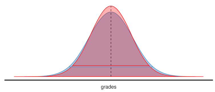
The first was this paper by Rose O'Dea, Malgorzata Lagisz (both UNSW), Michael Jennions (ANU), and Shinichi Nakagawa (UNSW), published in the journal Nature Communications. O'Dea and Nakagawa wrote about the paper in The Conversation late last month. The paper was based on a meta-analysis (an analysis that combined the results from many different studies into a single analysis) of 227 other studies that included over 1.6 million high school students. It tested the 'variability hypothesis' - the idea that male students in STEM (Science, Technology, Engineering, and Maths) subjects show greater variability in performance. That means that there are more male students than female students in each tail of the distribution - more male students than female students do very poorly, and more male students than female students do very well. So, you can think of the distributions of male and female students' grades as something like this:

The blue distribution (males) has a smaller peak and fatter tails than the red distribution (females), so there are more male students at the top of the distribution. Note that the distributions have the same mean, which is not what we would expect, since female students on average tend to do better. O'Dea et al. confirm that result, but also find some support for the variability hypothesis:

Overall, girls had significantly higher grades than boys by 6.3%... with 10.8% less variation among girls than among boys...

Girls’ significant advantage of 7.8% in mean grades in non-STEM was more than double their 3.1% advantage in STEM... Variation in grades among girls was significantly lower than that among boys in every subject type, but the sexes were more similar in STEM than non-STEM subjects...

In other words, girls had higher grades than boys in both STEM and non-STEM subjects, but the difference in the variability in grades was higher for non-STEM, not STEM, subjects. Here's the resulting distributions:

The ratio of female to male students is equal to one (equal numbers of female and male students) in the top 10% of the distribution of STEM grades, and in the top 2% of non-STEM grades. For the top X% of grades below those thresholds, there are more female than male students (and above those thresholds, there are more male than female students).

Essentially, based on these results, female students outperform male students in both STEM and non-STEM, but they outperform male students by more in non-STEM than in STEM. Which makes these results complementary to those of the second article, by Gijsbert Stoet (Leeds Beckett University) and David C. Geary (University of Missouri), published in the journal Psychological Science (gated, but for the moment at least, this link appears to take you directly to the PDF). Stoet and Geary use PISA (Programme for International Student Assessment) data from over 472,000 students from 67 countries, to look at the intra-individual academic strengths of male and female high school students. Basically, for each student they calculated whether the student performs better (or worse) in reading, maths, or science, compared with the other two subject areas, and by how much better (or worse) they did. They then compare those results between male and female students. They found that:

...there were consistent sex differences in intraindividual academic strengths across reading and science. In all countries except for Lebanon and Romania (97% of countries), boys’ intraindividual strength in science was (significantly) larger than that of girls... Further, in all countries, girls’ intraindividual strength in reading was larger than that of boys, while boys’ intraindividual strength in mathematics was larger than that of girls. In other words, the sex differences in intraindividual academic strengths were near universal...

We found that on average (across nations), 24% of girls had science as their strength, 25% of girls had mathematics as their strength, and 51% had reading. The corresponding values for boys were 38% science, 42% mathematics, and 20% reading.

In other words, female students' relative strength was more likely to be in reading, while male students' strength was more likely to be in science or mathematics. They also found that male students were more likely to overestimate their ability in science than female students were.

Alex Tabarrok at Marginal Revolution has the best take on Stoet and Geary's results:

Now consider what happens when students are told. Do what you are good at! Loosely speaking the situation will be something like this: females will say I got As in history and English and B’s in Science and Math, therefore, I should follow my strengthens and specialize in drawing on the same skills as history and English. Boys will say I got B’s in Science and Math and C’s in history and English, therefore, I should follow my strengths and do something involving Science and Math.

Note that this is consistent with the Card and Payne study of Canadian high school students that I disscused [sic] in my post, The Gender Gap in STEM is NOT What You Think. Quoting Card and Payne:

"On average, females have about the same average grades in UP (“University Preparation”, AT) math and sciences courses as males, but higher grades in English/French and other qualifying courses that count toward the top 6 scores that determine their university rankings. This comparative advantage explains a substantial share of the gender difference in the probability of pursing a STEM major, conditional on being STEM ready at the end of high school."

and myself:

"Put (too) simply the only men who are good enough to get into university are men who are good at STEM. Women are good enough to get into non-STEM and STEM fields. Thus, among university students, women dominate in the non-STEM fields and men survive in the STEM fields."

So, even though female students may be better than male students in STEM subjects at school, we may see fewer of them studying those subjects at university (let alone taking them as a career), because female students are also better in non-STEM subjects at school, and they are better by more in non-STEM than in STEM, compared with male students. Economists refer to this as the students following their comparative advantage. Female students have a comparative advantage in non-STEM, and male students have a comparative advantage in STEM subjects. That is different from absolute advantage (which female students appear to have in both subject areas, at least according to O'Dea et al. - the gender differences in average results are not consistently significant in Stoet and Geary). The O'Dea et al. results and the Stoet and Geary results both support this comparative advantage interpretation.

One final result from Stoet and Geary still needs further exploration. They report that:

...the relation between the sex differences in academic strengths and college graduation rates in STEM fields is larger in more gender-equal countries.

That is a surprising result. If we thought that making genders more equal would reduce the gender gap in STEM, we would expect the exact opposite result! Stoet and Geary's proffered explanation for this seems particularly weak:

Countries with the highest gender equality tend to be welfare states (to varying degrees) with a high level of social security for all its citizens; in contrast, the less gender-equal countries have less secure and more difficult living conditions, likely leading to lower levels of life satisfaction...

So, because people feel more secure in countries with better welfare states, which are also the countries with higher gender equality, they are less likely to pursue the high-risk, high-reward jobs in STEM fields, than safer jobs in non-STEM fields. That definitely needs more follow-up research.

Read more:

• STEM-readiness and the gender gap in STEM at university

Price discrimination and airline tickets

Earlier this month, Rob Nicholls (UNSW) wrote an article on The Conversation about airline ticket prices:

Few things are more annoying than spending a large sum of money on a purchase, only to discover that someone else got the same thing for a lower price. This often happens with airfares. You go the same website, search the same airline, choose the same seat row and fare conditions, but you’re offered a different price depending on when and where you do it. Why?

Often it’s a result of price discrimination. This happens when a seller charges you what you’re willing to pay. Of course, it also needs to be at a level that the seller is willing to accept.

When it comes to airfares, there are two levels of price discrimination, both driven by algorithms. First, there is price discrimination by the airline. Airline pricing is typically dynamic. That is, the prices are higher for more popular flights. Then there are intermediary platforms, such as travel agents or price comparison websites, which can introduce a further level of price discrimination.

Nicholls' article is interesting, but it misses some important points about the price discrimination undertaken by airlines, and so it is worth also considering those points. First, price discrimination only occurs when the seller is selling the same product to different consumers for different prices, and where those differences in prices don't reflect differences in cost. So, the difference in price between premium economy airline tickets and economy airline tickets is not price discrimination, because there are differences in cost between those ticket classes.

Second, perfect price discrimination (first degree price discrimination, or personalised pricing) is when a seller charges you exactly what you're willing to pay. However, sellers typically don't know what you're willing to pay (you might not even know what you're willing to pay), so most sellers engage in some form of imperfect price discrimination.

In contrast, third degree price discrimination (group pricing) occurs when the sellers charges different prices to different known groups of consumers. This is the type of price discrimination that movie theatres engage in, when they sell the same tickets to students or seniors for a lower price than general admission. This isn't the type of price discrimination that airlines engage in.

Airlines typically engage in second degree price discrimination. This is where the sellers doesn't know the willingness to pay of the consumer, and doesn't know what group they belong to, but they can infer from the consumer's choices how much they are willing to pay. One type of second degree price discrimination is menu pricing. It's called menu pricing, because it is the type of pricing that restaurants use. The seller offers a menu of different options, and knows which options will appeal to consumers with relatively inelastic demand (where the mark-up should be higher), and other options will appeal to consumers with relative elastic demand (where the mark-up should be lower).

Airlines don't quite have a menu. However, they do offer a range of options to consumers. Some consumers will buy a ticket close to the date of the flight, while others buy far in advance. That is information the airline can use. If you are buying close to the date of the flight, the airline can assume that you really want to go to that destination on that date, and that few alternatives will satisfy you (maybe you really need to go to Canberra for a meeting that day, or to Christchurch for your aunt's funeral). Your demand will be relatively inelastic, so the airline can increase the mark-up on the ticket price. In contrast, if you buy a long time in advance, you probably have more choice over where you are going, and when. Your demand will be relatively elastic, so the airline will lower the mark-up on the ticket price. This intertemporal price discrimination is why airline ticket prices are low if you buy far in advance.

Similarly, if you buy a return ticket that stretches over a weekend, or a flight that leaves at 10am rather than 6:30am, you are more likely to be a leisure traveller (relatively more elastic demand) than a business traveller (relatively more inelastic demand), and will probably pay a lower price.

The outcome, as Nicholls notes, is that you are unlikely to be paying the same ticket price as the person seated next to you on the plane. The ticket price you paid will be based on the airline's assessment of your willingness to pay, based on the choices you have made.

Russ Roberts on the income distribution

Students in my ECONS102 class would have gotten the message in the last week of classes that much of the rhetoric (in New Zealand, at least) around inequality is somewhat misleading, if not just plain wrong. For example: "Inequality is getting worse over time". No, it's not. At least, not in New Zealand since about the mid-1990s (the data supports this - there are any number of posts by Eric Crampton that show it, but try this one for starters). You might believe that inequality is a Bad Thing, but you don't need to overstate your case - inequality can be a Bad Thing even if it is not getting worse.

In a new article on Medium, Russ Roberts takes aim at another data fallacy:

Adjusted for inflation, the US economy has more than doubled in real terms since 1975.

How much of that growth has gone to the average person? According to many economists, the answer is close to zero...

But the biggest problem with the pessimistic studies is that they rarely follow the same people to see how they do over time. Instead, they rely on a snapshot at two points in time. So for example, researchers look at the median income of the middle quintile in 1975 and compare that to the median income of the median quintile in 2014, say. When they find little or no change, they conclude that the average American is making no progress.

But the people in the snapshots are not the same people...

Studies that use panel data — data that is generated from following the same people over time — consistently find that the largest gains over time accrue to the poorest workers and that the richest workers get very little of the gains. This is true in survey data. It is true in data gathered from tax returns...

One explanation of these findings is there is regression to the mean — if your parents are particularly unlucky, they may find themselves at the bottom of the economy. You, on the other hand, can expect to have average luck and will find it easier to do better than your parents. At the other end of the income distribution, one reason you might have very rich parents is that they have especially good luck. You are unlikely to repeat their good fortune, so you will struggle to do better than they did.

To see the problem with the pessimistic studies, consider a very simple economy with just three people. In 2005, Anna has income of $10,000, Bill has income of $20,000, and Charlotte has income of $70,000. The median income is $20,000. The total income of the bottom two-thirds of the population is $30,000. The lowest one third of the population (Anna) earns only one seventh of the earnings of the top one third of the population (Charlotte).

Now, say you collect some data on these same people ten years later, and find that Anna now has income of $20,000, Bill has income of $80,000, and Charlotte has income of $5,000. The median income is still $20,000. The median income is still $20,000. The total income of the bottom two-thirds of the population has decreased from $30,000 to $25,000. The lowest one third of the population (Charlotte) earns only one sixteenth of the earnings of the top one third of the population (Bill). If you ignored the dynamics of the income changes, you would either conclude that lower-income people are no better off than ten years earlier (the median income has not changed), or that they are worse off (lower total earnings, or higher inequality). But that would ignore the fact that two-thirds of the population is actually better off than before.

Comparing cross-sections over time is fraught, and the potential for drawing erroneous conclusions is high. As Russ Roberts concludes:

If we want to give all Americans a chance to thrive, we should understand that the standard story is more complicated than we’ve been hearing. Economic growth doesn’t just help the richest Americans.

And unlike much of what we read about incomes and inequality in the U.S., Roberts' conclusion is probably true for New Zealand as well.

[HT: Marginal Revolution]

Why Waiheke Island taxi drivers are like surfers

This New Zealand Herald article caught my eye this week:

Two Auckland-based taxi drivers claim they have been subjected to bullying, racist remarks and had their tyres slashed by local drivers while working on Waiheke Island.

Waiheke Island-based companies Island Taxis and Waiheke Five-O say there's been a recent spike in the numbers of "pirate" Auckland drivers bringing their cars over on the ferry and poaching business off them at weekends.

Island Taxis driver Richard Cannon told the Herald seven or eight drivers had been "clogging up the rank" at the Matiatia Wharf ferry terminal and poaching "about a third" of local drivers' income.

Taxi ranks are what economists refer to as a 'common resource'. They are rival (one taxi driver parking on the taxi rank reduces the amount of space available for other taxis), and non-excludable (it isn't easy to prevent taxis from parking at the rank). The problem with common resources is that, because they are non-excludable (open access), they are over-consumed. In this case, there will be too many taxis (including taxis from the mainland) competing for taxi rank places (and customers) on Waiheke Island.

The solution to the problem of common resources is somehow to convert them from open access to closed access. That is, to somehow make them excludable. And it seems that is what the vigilante actions of the Waiheke drivers is aiming to do - to exclude the mainlander taxi drivers from operating.

This is very similar to how surf gangs operate to exclude some surfers (particularly those who are not locals) from the best surfing spots, as I have blogged about before (see here and here). There is no government intervention to manage the common resource, so it is up to the user community (taxi drivers) to do so. As 2009 Nobel Prize winner Elinor Ostrom noted, this requires that the user community can form a homogeneous group (within which trust is high), with common goals for the resource (in this case the taxi rank); and that both the boundary of the resource and of the community are well defined. Local taxi drivers are a (relatively) homogeneous group, and the boundary of the resource (taxi rank and customers) and the community (taxi drivers must be licensed) are well defined. But only until the outsiders come in, at which point the group is no longer homogeneous, and the previous private solution to the common resource problem breaks down. Resulting in violence between local taxi drivers and mainlanders, which is similar to surf gang violence.

Read more:

• New research coming on surf rage in New Zealand
• The escalation of surf gang violence

It may be a good time to buy a car

Given that my ECONS101 students have their final exam next week, a post on supply and demand seems timely. Let's consider this New Zealand Herald article from last week:

In a twist of irony, now might be the best time to buy a new car.

As rising fuel prices burn Kiwi wallets, the Vehicle Industry Association (VIA) has released a statement saying a glut of imported cars has created excessive supply, pushing down retail prices.

Consider the market for second-hand cars in New Zealand, as shown in the diagram below. Initially, the market is at equilibrium, where the demand curve D0 meets the supply curve S0. The equilibrium price is P0 and the equilibrium quantity is Q0.

Then, there is an increase in supply (from S0 to S1). The article mentions that this is because:

"The stink bug disrupted car importing for a lot of dealers earlier this year and left them waiting longer than usual for stock while vehicles were treated for the pest and held up at our borders," [Trade Me spokesperson Millie] Silvester said.

"Now this backlog has cleared and so as a result we've seen a flood of vehicles come onto site."

At the same time, there has probably been a decrease in demand. Why? Petrol and cars [*] are complements. If you have a car, it needs petrol. The petrol price has been increasing recently. Consumers will respond by demanding less petrol, and by looking for alternatives to cars, so the demand for cars will reduce (from D0 to D1 on the diagram).

At the original equilibrium price of cars, there is now excess supply, or a surplus (the quantity supplied (QS) is greater than the quantity demanded (QD)) - sellers can't sell all of the cars they have at that high price. You can expect the price of cars to fall (eventually settling at the new equilibrium price, P1). So, it might be a good time to buy a car.

What has happened to the quantity of cars traded? When we know there is a decrease in demand and an increase in supply, we can be sure the equilibrium price will decrease, but the change in equilibrium quantity is ambiguous, because it depends on the relative size of the shifts in supply and demand (if supply has increased by more than the decrease in demand, the equilibrium quantity will increase; but if demand has decreased by more than the increase in supply, the equilibrium quantity will decrease). In this case, the increase in supply seems to be larger than the decrease in demand, because the article notes that:

"Retail car sales (including imports) have been tracking well for us. In fact, we just had our best ever retail volume month and we are very confident as we come into the summer months which are normally quite buoyant for our business," [Turners chief executive Greg] Hedgepeth said.

*****

[*] At least, petrol and petrol-powered cars are complements. Electric cars will be substitutes for petrol and petrol-powered cars, but they are still only a small share of the market.

Book Review: Fifty Inventions that Shaped the Modern Economy

I really enjoy Tim Harford's writing, on his blog, and in his previous books (here are my reviews of Adapt, The Undercover Economist Strikes Back, and Dear Undercover Economist). So, I've been looking forward to reading his latest book, Fifty Inventions that Shaped the Modern Economy, for some time. And it didn't disappoint. When you read a book that is really a long list of things, there is a real risk that it devolves into one of the dime-a-dozen listicles that pervade the internet. Harford avoids that trap because of his engaging writing style, and the ability to link together anecdotes and stories into a supremely readable whole. Consider the following passage, in the chapter on cuneiform:

The Egyptians also thought that literacy was divine, a benefaction from baboon-faced Thoth, the god of knowledge. Mesopotamians thought the goddess Inanna had stolen it for them from Enki, the god of wisdom - although Enki wasn't so wise that he hadn't drunk himself insensible...

Scholars no longer embrace the "baboon-faced Thoth" theory of literacy.

It's just as well. The book isn't a collection of the fifty most important inventions, or the fifty most profitable inventions, or even the welfare-enhancing inventions. Harford omits some obvious candidates in those categories, such as fire, or the wheel. However, the list includes a number that you might not have considered yourself until you read about them, such as passports, the barcode, or property registers. The chapter on double-entry bookkeeping was a surprising highlight, as was the chapter on the s-bend, which includes this bit:

Flushing toilets had previously foundered on the problem of smell: the pipe that connects the toilet to the sewer, allowing urine and feces to be flushed away, will also let sewer odors waft back up - unless you can create some kind of airtight seal.

Cumming's solution was simplicity itself: bend the pipe. Water settles in the dip, stopping smells from coming up; flushing the toilet replenishes the water. While we've moved on alphabetically from the S-bend to the U-bend, flushing toilets still deploy the same insight: Cumming's invention was almost unimprovable.

Not all of the inventions are positive - the book includes chapters on tax havens, antibiotics in farming, and plastics (seen as good at the time, but not so much now) - but all have been transformative in their own way. The lightbulb, which we associate with ideas, appears only in the last chapter.

This is an excellent book, well-researched and interesting throughout. I found it hard to put down, and I'm sure many of you will also. Recommended!

The economics of trademark protection

Last week, William Nordhaus won the Nobel Prize in economics and as I mentioned at the time, one of his contributions to economics was a recognition of the trade-offs inherent in the protection of intellectual property rights. Strong intellectual property rights provide an incentive for investment in creation or development of new intellectual property, but they also provided a limited monopoly to the holder of the intellectual property rights. The trade-off (as we'll see a little later in this post) is between under-creation of intellectual property if there is weak protection, and under-consumption of the intellectual property if there is strong protection.

Intellectual property rights can be protected through patents or copyright, or through trademarks as this article from last week notes:

Trademark protection is available to businesses of all sizes and there are very good reasons for traders to use that protection...

The registered owner is deemed to have the exclusive right to use the mark throughout New Zealand in relation to all the goods and services it covers; the owner's rights are on a publicly searchable register, which may have a deterrent effect on copy-cats; and it has the right to sue under the the [sic] Trade Marks Act 2002...

...the trademark system also has wider economic benefits.

Providing legal protection for brands incentivises businesses to invest in building goodwill and reputation by producing high quality goods and services.

Trademarks provide an incentive for Firm A to invest in building goodwill, because Firm A's goodwill can't be captured by other firms that are pretending to sell Firm A's goods. Consider the diagram below, which shows the market for a firm selling a trademarked product. The trademark makes the firm a monopoly (in this particular trademarked product). It gives the firm some market power. The trademark is costly to obtain (it involves the cost of the trademark itself, but also the cost of building consumer awareness of the brand the trademark protects), and that fixed cost leads to some economies of scale. This is why the average cost (AC) curve is downward sloping. If the firm is maximising its profits, it will operate at the point where marginal revenue meets marginal cost, i.e. at the quantity QM, which it can obtain by setting a price of PM (this is because at the price PM, consumers will demand the profit-maximising quantity QM). The firm makes a profit that is equal to the area PMBKL. [*]

Now consider what would happen if there was no trademark protecting the product. Other competing firms would realise that this product is quite profitable, and they would start to sell it (since there is no trademark stopping them from doing so). We end up with a market that is more competitive, which would operate at the point where supply (MC) meets demand. This is at a price of PC, and the quantity of QC. Notice that the price is now below average cost - the firm that developed the product sells at a loss (equal to the area JFEPC). [**]

So, if there is strong intellectual property rights protection (trademarks in this case, but a similar analysis applies to patents or copyright), there would be less consumption of intellectual property (because QM is much less than QC). But, if there is weak intellectual property rights protection, there would be less development of intellectual property in the first place (because the developer would face the costs of development, but could not easily profit from it).

Trademarks are clearly valuable for firms, but the article also argues that they are valuable for consumers:

Trademark protection also has a consumer welfare aspect. Trademarks are "badges of origin" for consumers, a sort of guarantee to indicate that a product or service comes from a trusted, reliable source.

Regulating their use (and misuse) helps to protect the buying public from confusion and, at worst, physical harm.

At the extreme end of the spectrum, counterfeit products can pose an active risk to health.

Last month, the BBC reported hundreds of thousands of pounds of counterfeit cosmetics had been seized in the UK, some of which contained chemicals such as highly toxic mercury and the illegal levels of the skin-whitening agent hydroquinone.

Intellectual property rights is an interesting topic that I cover in my ECONS102 class, particularly because it involves a difficult trade-off. It isn't clear how strong intellectual property rights protection should be, in order to balance under-consumption (relative to an economic-welfare-maximising point) against under-development (because of the lack of profits from developing intellectual property). Clearly, we still don't have the balance right if we are still facing drug pricing that works like this.

*****

[*] This is different from the producer surplus, which is the area PMBHPC. The difference between producer surplus and profits arises because of the fixed cost - in this case, the cost of the trademark and product development.

[**] The producer surplus in this case is zero. This is because the diagram shows a 'constant cost' firm, where marginal cost is constant (so every unit costs the same to produce), and the equilibrium price is equal to marginal cost. Also, more realistically if you don't create the trademark in the first place, the fixed cost is eliminated. So there is no loss, but there is also no profit because every unit is sold at its marginal cost.

Book Review: The Company of Strangers

If you've been reading about economics for long enough, sooner or later you will come across reference to the miracle that is the production of a lead pencil. Perhaps you'll read about it in the context of a Milton Friedman interview (like here), or perhaps a reference to the original, Leonard Read's 1958 book I, Pencil (see here). Either way, the story is about spontaneous order and/or interdependence - how the actions of hundreds or more people interact produce a single pencil, without any one of them necessarily caring about the end product, or even knowing how it is produced.

Over the years, I've seen several references to Paul Seabright's book, The Company of Strangers, in a similar context to I, Pencil. So, I finally took the time to read it (or rather, the revised edition from 2010 - the original was published in 2001). The essence of the book can be summarised as follows, from the introduction to the book:

• First, the unplanned but sophisticated coordination of modern industrial societies is a remarkable fact that needs an explanation. Nothing in our species' biological evolution has shown us to have any talent or taste for dealing with strangers.

• Second, this explanation is to be found in the presence of institutions that make human being willing to treat strangers as honorary friends.

• Third, when human beings come together in the mass, the unintended consequences are sometimes startlingly impressive, sometimes very troubling.

• Fourth, the very talents for cooperation and rational reflection that could provide solutions to our most urgent problems are also the source of our species' terrifying capacity for organized violence between groups. Trust between groups needs as much human ingenuity as trust between individuals.

Trust is central to the modern economy, and has been central to social interactions for as long as Homo sapiens has gathered into groups. In my ECONS101 class, I always wish we had more time to consider repeated games in our game theory topic, where trust and reputation become key features of the resulting outcomes. 

The book is thoroughly researched and very deep. Seabright draws from a range of sources from biology to anthropology to economics. Every paragraph made me think, which made for a long read (in case you were wondering why I haven't posted a book review since early September). Seabright also provided me with a number of novel ways of explaining some key concepts in my classes.

Some readers may find the book quite dry, but there are also some lighter highlights, such as this:

There is a lost look sometimes that flits across the brow of those senior politicians who have not managed to attain perfect facial self-control. It is the look of a small boy who has dreamed all his life of being allowed to take the controls of an airplane, but who discovers when at last he does that none of the controls he operates seems to be connected to anything, or that they work in such an unpredictable way that it is safer to leave them alone altogether. Politicians have very little power, if by power we mean the capacity to achieve the goals they had hoped and promised to achieve.

If only more politicians, and voters, understood this point! And this as well:

As the twenty-first century develops, "globalization" has become a convenient catch-all term to sum up the multitude of different, often contradictory reasons people have to feel uneasy about the way in which world events are developing.

Since the book is really about trust between people, and globalization is ultimately about connections between people, there are some good underlying discussions to be found in its pages. Seabright also provides an interesting perspective on the Global Financial Crisis (which was contemporary at the time of writing the revised edition). However, at its heart this is a book about people, and our interactions in a world where we don't know the majority of people with whom we interact. Like spontaneous order, such interactions are at the heart of economics. If you want to develop a deeper understanding of these interactions, this book would be a good one to read.

Petrol prices and drive-offs

The New Zealand Herald reported yesterday:

Due to increasing costs of crude oil, the New Zealand dollar falling and increasing fuel taxes, petrol pumps are forcing a strain on Kiwis.

Some motorists are taking drastic actions to avoid the economic sting, putting in fuel and driving away from stations before paying.

Over the last few weeks, Z Energy has witnessed a small increase of motorists getting behind the wheel instead of the cash register.

"At a high level we have seen a slight increase in the number of drive-offs," a spokeswoman said.

Why the increase in drive-offs? Gary Becker (1992 Nobel Prize winner) argued that criminals are rational, and they would weigh up the benefits and costs of their actions (see the first chapter in this pdf). It is rational to execute a drive-off if the benefits of the drive-off (the savings in fuel costs because they fuel wasn't paid for) exceed the costs of the drive-off (the penalty for being caught, multiplied by the probability of being caught).

How often will people engage in drive-offs? We can think about that question in terms of the marginal benefits and marginal costs of drive-offs, as shown in the diagram below. Marginal benefit (MB) is the additional benefit of engaging in one more drive-off. In the diagram, the marginal benefit of drive-offs is downward sloping - the first drive-off provides a relatively high benefit (filling an empty tank), but subsequent drive-offs will likely provide less additional benefit, because the car's tank is already close to full. Marginal cost (MC) is the additional cost of engaging in one more drive-off. The marginal cost of drive-offs is upward sloping - the more drive-offs a person engages in, the more likely they are to get caught. The 'optimal quantity' of drive-offs (from the perspective of the person engaging in the drive-offs!) occurs where MB meets MC, at Q* drive-offs. If the person engages in more than Q* drive-offs (e.g. at Q2), then the extra benefit (MB) is less than the extra cost (MC), making them worse off. If the person engages in fewer than Q* drive-offs (e.g. at Q1), then the extra benefit (MB) is more than the extra cost (MC), so conducting one more drive-off would make them better off.

Now consider what happens in this model when the price of petrol increases. The benefits of drive-offs increase, because the value of fuel cost savings from driving off increases. As shown in the diagram below, this shifts the MB curve to the right (from MB0 to MB1), and the optimal quantity of drive-offs increases from Q0 to Q1. Drive-offs increase.

Regular readers of this blog will recognise that this situation is quite similar to the increase in honey thefts reported earlier this year. Petrol prices are expected to increase further through the rest of this year. Petrol stations should be preparing themselves for increases in drive-offs. Consumers can probably expect more petrol stations to move to having their pumps on pre-pay.

Read more:

• Why honey thefts are on the rise

Nobel Prizes for Paul Romer and William Nordhaus

The 2018 Sveriges Riksbank Prize in Economic Sciences in Memory of Alfred Nobel (aka Nobel Prize in Economics) has been awarded to William Nordhaus of Yale "for integrating climate change into long-run macroeconomic analysis" and Paul Romer of NYU "for integrating technological innovations into long-run macroeconomic analysis."

Marginal Revolution has excellent coverage as always, on Nordhaus and on Romer. Romer's work on endogenous growth theory hasn't had much influence on my teaching as I don't teach macroeconomics or growth, but here is an excellent video from MRU that summarises many of the key contributions:

As you might expect, Nordhaus' work on the economics of climate change is picked up in my ECONS102 class in the topic on externalities and common resources. Here is my review of his book The Climate Casino - it's good that I finally read a laureate's most recent book before they received the award for once! Nordhaus has also contributed to our understanding of the economics of intellectual property rights, which Marginal Revolution didn't mention, but which I have talked about briefly here and here. His approach, in terms of the trade-off between having weaker (or shorter) intellectual property rights, which would lead to under-investment in intellectual property development, or having stronger (or longer) intellectual property rights, which would lead to under-consumption of intellectual property, is what I follow in teaching that topic in ECONS102.

This was a very well deserved (and overdue) prize for both men. However, I was a little surprised that they shared the prize together (in the Economics Discussion Group poll, both this year and last year, I picked Romer and Robert Barro to win). Nonetheless, an excellent choice.

The effect of cutting subsidies for after-hours doctors

The New Zealand Herald reported last week:

Parents who received free after-hours medical care for their children are now having to pay up to $61 at two Auckland clinics following funding cuts from district health boards...

The changes meant White Cross Glenfield's casual fee for under 13s after hours skyrocketed from free to $61.

At Three Kings Medical Centre, prices for care after 5pm had gone up to $50 for children aged between 6 to 12 - and $35 for under-6-year-olds.

This is what happens when you remove a subsidy - the price that consumers pay goes up. To see why, consider the market in the diagram below. The subsidy is paid to the supplier (the after-hours medical clinic), so we show it using the S-subsidy curve. The consumers (patients) pay the price where that curve meets the demand curve (PC), which from the article above could be as low as zero. The clinic receives that price (PC) from the patient, but then is topped up by the government subsidy, and receives an effective price of PP. The number of patients going to the clinic is Q1. If the subsidy is removed, the market shifts to equilibrium, where demand meets supply. The price for patients increases to P0, and the price received by clinics decreases to P0. The number of patients going to the clinic decreases to Q0.

The article notes that the subsidy hasn't been removed from all clinics. So, patients may simply go to some other clinic instead of the nearest one, if the nearest one is no longer subsidised. This was effectively what the DHB was trying to achieve:

Waitemata and Auckland City DHB announced a rejig to after-hours clinic funding in July in a bid to "reduce inequalities".

Presumably, that means that the DHB removed the subsidies from clinics in areas that are relatively more affluent (so that a higher proportion of the total subsidy goes to areas that are less affluent)? A more cynical view is that the DHB will benefit from some cost savings (which they may need!). The cost savings arise because fewer patients in total will go to after-hours clinics that are subsidised (if your illness isn't urgent or critical, maybe you choose not to go to the doctor, because the subsidised clinic is far away, and the unsubsidised clinic is now more expensive). The DHB also benefits from administration cost savings, because the DHB now has to deal with fewer clinics. The costs of the removed subsidy are borne by patients (their medical care is now more expensive, because it is unsubsidised, or because they have to travel further to get to a subsidised clinic) and the now-unsubsidised clinics (who receive a lower effective price from patients, and see fewer of them).

Another way of looking at who is made worse off by removing this subsidy is to consider economic welfare. Consumer (patient) surplus is the difference between what consumers are willing to pay for the service (shown by the demand curve) and the price they actually pay. In the diagram above, the consumer surplus is the triangle AEPC when there is a subsidy, but decreases to ABP0 when the subsidy is removed. Consumers (patients) are worse off without the subsidy.

Producer (clinic) surplus is the difference between the price that the producers receive and the producers' costs (shown by the supply curve). In the diagram above, the producer surplus is the triangle PPFG when there is a subsidy, but decreases to P0BG when the subsidy is removed. Producers (clinics) are worse off without the subsidy.

The taxpayer (the DHB) is the only party made better off without the subsidy. [*]

Finally, the loss of economic welfare is not the only cost of the removal of the subsidy. If patients are dissuaded from attending a clinic at all because of the higher cost, there could be real health losses that arise from the change in policy. It would be interesting to know how big an effect this has.

*****

[*] I have ignored what happens to total economic welfare in this diagram and this analysis. Typically, if we draw a subsidy on a market and the subsidy moves the market away from the quantity where marginal social benefit is equal to marginal social cost (as in the diagram I have shown), total economic welfare decreases (the subsidy makes society worse off, on aggregate). However, health care has positive externalities that are also not represented in the diagram, and in the presence of positive externalities a subsidy can actually increase (rather than decrease) total economic welfare. I've opted to keep the diagram simple by ignoring positive externalities and the effect on total welfare.

Why study economics? Economists in tech companies edition...

In my ongoing series of posts entitled "Why study economics?" (see the end of this post for links), several times I have highlighted the increasing role of economists in technology companies. In a new NBER Working Paper (ungated version here), Susan Athey (previously chief economist at Microsoft, and now at Stanford and on the board of a number of technology companies) and Mike Luca (Harvard) provide a great overview of the intersection of economics (and economists) and technology companies:

PhD economists have started to play an increasingly central role in tech companies, tackling problems such as platform design, pricing, and policy. Major companies, including Amazon, eBay, Google, Microsoft, Facebook, Airbnb, and Uber, have large teams of PhD economists working to engineer better design choices. For example, led by Pat Bajari, Amazon has hired more than 150 Ph.D. economists in the past five years, making them the largest employer of tech economists. In fact, Amazon now has several times more full time economists than the largest academic economics department, and continues to grow at a rapid pace.

Importantly, it isn't just PhD economists:

Tech companies have also created strong demand for undergraduate economics majors, who take roles ranging from product management to policy.

What is it about economics that creates value for tech firms? Athey and Luca identify:

...three broad skillsets that are part of the economics curriculum that allow economists to thrive in tech companies: the ability to assess and interpret empirical relationships and work with data; the ability to understand and design markets and incentives, taking into account the information environment and strategic interactions; and the ability to understand industry structure and equilibrium behavior by firms.

One further interesting point is that:

...Amazon was the largest employer of Harvard Business School’s most recent graduating class of MBA students.

The job market for economics graduates (or, more broadly, graduates with skills in economics) is looking stronger.

[HT: Marginal Revolution]

Read more:

• Why study economics? Uber data scientist edition...
• Why study economics? Better than operations research and computer science edition...
• Why study economics? Economics and computer science edition...
• Why study economics? Understand the world edition...
• Why study economics? More tech sector jobs edition...
• Why study economics? Law and economics edition...
• Why study economics? More on jobs in the tech sector edition...
• Why study economics? Tech firm jobs edition...
• Why study economics? AEA video edition...
• Why study economics? Even if you won't be an economist edition...
• Why study economics? PhD edition...
• Why study economics? It could make you rich...
• Why study economics? Sheepskin effects edition
• Why study economics? NZ graduate earnings edition
• Why study economics?

Your Fitbit will betray you

Yesterday I wrote a post about how home insurers are starting to more accurately price house insurance based on natural hazard risk. Home insurance isn't the only area where insurers are looking at adopting more sophisticated screening methods to deal with adverse selection. Take this story from the New Zealand Herald in June:

Fitbits are already used to track your heart rate, the amount of exercise you do and how much you sleep - essential data that could potentially be used by insurance providers to determine your premiums.

The boom in wearable health tracking technology means we now have more information than ever before on health and well being of people at any given moment.

The Telegraph reports that information collected from these devices is already being used by insurers to calculate insurance premiums and there are concerns that this might lead to only the healthiest customers enjoying lower premiums.

This is serious business. Insurance companies have it in their interests not only to ensure the lowest-risk customers but also to detect potential health conditions before they become severe (and expensive). A study of the insurance market by the Swiss Re Institute, a research organisation, last year found that insurers had filed hundreds of patent applications relating to "predictive insurance modelling".

The issue that an uninformed health insurer or life insurer faces is essentially the same as the home insurer from yesterday's post. They can't tell the low-risk applicants from high-risk applicants. A pooling equilibrium develops, where everyone pays the same premiums (coarsely differentiated based on age, gender, and smoking status). A savvy and entrepreneurial insurer that was better able to tell who the low-risk insured people are could attract them away with lower premiums (knowing that they would cost less to insure because they are low risk).

So, that is effectively what insurers are starting to do. As the Herald article notes:

In making these moves, Insurance companies aim to collect data that could serve to help them make better policy decisions or even tweak existing policies over time.

The Telegraph reported that policy agreements increasingly feature clauses that allow insurers to collect data on their customers.

This is a point that I first made in a post back in 2015 (and an earlier post on technology in car insurance in 2014). We can all look forward to insurers asking for our Fitbit data when we apply for health or life insurance. And if we're fit and healthy, we'll give it to them. The people most likely to withhold that information are the unfit and unhealthy (and those who are most privacy-conscious). Denying access to your Fitbit data would probably be enough to signal to the insurer that you are high risk, and result in a declined application or a higher premium. So, even if you want to opt out of sharing your data, your Fitbit will still betray you.

Read more:

• The most surprising thing I learned about home insurance this year
• Why your Fitbit or Apple Watch could soon get you cheaper health insurance
• Could technology eliminate moral hazard in car insurance?
• Is there adverse selection in the life insurance market?

The most surprising thing I learned about home insurance this year

Home insurance markets are subject to adverse selection problems. When a homeowner approaches an insurer about getting home insurance, the insurer doesn't know whether the house is low-risk or high-risk. [*] The riskiness of the house is private information. In fact, the riskiness of the house is probably not known even to the homeowner, but let's assume for the moment that they have at least some idea. To minimise the risk to themselves of engaging in an unfavourable market transaction, it makes sense for the insurer to assume that every house is high-risk. This leads to a pooling equilibrium - low-risk houses are grouped together with the high-risk houses and owners of both types of house pay the same premium, because they can't easily differentiate themselves. This creates a problem if it causes the market to fail.

The market failure may arise as follows (this explanation follows Stephen Landsburg's excellent book The Armchair Economist). Let's say you could rank every house from 1 to 10 in terms of risk (the least risky are 1's, and the most risky are 10's). The insurance company doesn't know who is high-risk or low-risk. Say that they price the premiums based on the 'average' risk ('5' perhaps). The low risk homeowners (1's and 2's) would be paying too much for insurance relative to their risk, so they choose not to buy insurance. This raises the average risk of the homes of those who do buy insurance (to '6' perhaps). So, the insurance company has to raise premiums to compensate. This causes some of the medium risk homeowners (3's and 4's) to drop out of the market. The average risk has gone up again, and so do the premiums. Eventually, either only highest risk homeowners (10's) buy insurance, or no one buys it at all. This is why we call the problem adverse selection - the insurance company would prefer to insure low-risk homes, but it's the homeowners with high-risk homes who are most likely to buy.

Of course, insurers are not stupid. They've found ways to deal with this adverse selection problem. When the uninformed party (the insurer in this case) tries to reveal the private information (about the riskiness of the house), we refer to this as screening. Screening involves the insurer collecting information about the house and the homeowner in order to work out how risky the house is. With the private information revealed, the insurer can then price accordingly - higher-risk houses attract higher premiums, while lower-risk houses attract lower premiums. We have a separating equilibrium (the high-risk and low-risk houses are separated from each other in the market).

With all this in mind, this story from April surprised me greatly:

Other insurers are likely to follow NZX-listed Tower's lead and increase their focus on risk-based pricing for natural hazards, says an insurance expert...

Thousands of home-owners who live in high-risk earthquake-prone areas and insure via Tower are set to face hikes in their premiums while those in low-risk areas like Auckland will get a cut.

The insurance company, which is New Zealand's third largest general insurer, said it would stop cross-subsidising its policy-holders from April 1 in a bid to send a clearer message to home-owners about the risks of where they lived.

Tower chief executive Richard Harding said at the moment six Auckland households were paying more to subsidise insurance premiums for every one high-risk house in Wellington, Canterbury or Gisborne.

In other words, insurers previously weren't screening for all available private information before pricing their insurance for a given house. Essentially, owners of low-risk houses have been paying premiums that are too high, and owners of high-risk houses have been paying premiums that are too low. It took a little while, but eventually other insurers have also started to use risk assessments in determining insurance premiums, so this discrepancy is disappearing.

Why didn't the market break down due to adverse selection? The issue here is something I noted earlier in the post - the riskiness of a house is private information to both the insurer and the homeowner. If the homeowner doesn't know how risky their house is, owners of low-risk houses can't tell if the insurer is pricing their insurance too high relative to the risk of natural hazard damage. So, the owners of low-risk houses have no reason to drop out of the market. And, if the owners of low-risk houses don't drop out of the market, insurers have no reason to raise premiums.

However, that leaves the market open to disruption. As noted in the April article:

Jeremy Holmes, a principal at actuarial consulting firm Melville Jessup Weaver, said it was hard to say how long this would take. Insurers needed to be as good as their competitors at distinguishing risk.

"Otherwise they risk having their competitors target the lower-risk policyholders whilst they are left with only the higher risks ..."

An entrepreneurial insurer that was able to distinguish the low-risk houses from high-risk houses could start approaching owners of low-risk houses and offering them lower premiums. The remaining insurers would be left with higher-risk houses on average, and would have to raise premiums. This would increase the number of homeowners dropping out of the market (or rather, going to the insurer that was pricing according to risk). Tower was the first insurer to shift to risk-based premiums, so presumably they recognised this issue before any of the other insurers and acted exactly as you would expect - by moving to risk-based premiums before any potential disruptor could enter the market.

Still, it's a little surprising (to me, at least) that pricing based on natural hazard risk wasn't already happening.

*****

[*] For simplicity, I'm going to refer to low-risk houses and high-risk houses, when risk is probably as much a function of location as of the house itself. So, if you must, read 'low-risk house' as 'house with a low risk of damage in an earthquake', and 'high-risk house' as 'house with a high risk of damage in an earthquake'.